Developing RonDB with Claude: Lessons from 30 Years of Database Engineering

After 30 years of developing MySQL NDB Cluster and RonDB, a new tool has fundamentally changed how I write code. Here is what I have learned about working with Claude on a large-scale distributed database project.

A New Era for Database Development

A while ago I got a new tool that completely changes the way I develop code. I have worked on developing MySQL NDB Cluster — and now the fork RonDB — for more than 30 years. Over that time, many of the original findings about software engineering have shifted. In the 1990s, I learned that unit testing was important. However, I quickly discovered that in a startup with limited resources, it was not feasible to write unit tests for distributed database functionality. I even wrote a tool for generating distributed unit test programs, but the overhead remained too high.

With Claude, this equation completely changes. I can now modify 1,000 lines of code in a day — often more — and in parallel, instruct Claude to write 3–5x as many lines of test code for comprehensive unit testing. Claude does not just improve my coding productivity; it also makes the path to high-quality code faster by enabling test coverage that was previously impractical.

Will AI Cause Unemployment?

Some ask a philosophical question: does this mean the world will see unemployment due to AI coding tools? Personally, I think not. For me, it simply means that features I have been wanting to build for 20+ years are now suddenly possible. The only reason for unemployment would be if humanity ran out of ideas for what to develop next. I do not believe that will ever happen — just look into space and realise that God's creation is far too vast for us to explore, even with 1,000x more compute power than we have today. There will always be a new thing to understand and develop around the next corner.

A Word of Caution

Not all my experiences with AI coding have been positive. We had a REST API server written in Go that needed to be ported to C++. The AI performed a straightforward translation, but this created significant performance issues and produced code that was unreadable unless you had studied every new C++ feature in the latest standard. The translation took two months; fixing the resulting issues took six months. In retrospect, writing the C++ implementation from scratch would likely have been more efficient than using AI translation.

The lesson: AI works best when you guide it with clear architectural direction, not when you use it for mechanical translation without oversight.

Getting Started: The RonDB CLI

My first real attempt at using Claude for RonDB was creating a CLI tool. A colleague initally created it and I developed it further. I realised how well-suited this type of boilerplate code was for AI assistance. I extended our REST API, added new CLIs for Rondis, the REST API, and even a MySQL client interface. This was straightforward work — it would have been fairly easy even without Claude — but it still would have taken two to three months. With Claude, it was done within a week.

The Big Challenge: Pushdown Join Aggregation

Encouraged by the CLI experience, I decided to tackle something far more ambitious. For over ten years, I had wanted to develop Pushdown Join Aggregation in NDB/RonDB. This feature would allow complex join queries with aggregation to execute directly in the data nodes rather than pulling data up to the MySQL Server. However, it was a task that would have taken a year or more, so it never rose high enough on the priority list. With Claude, I estimated I could complete it in one to two months.

Background

NDB/RonDB already had two key building blocks in place. First, Pushdown Join has been supported for a long time, enabling complex join queries to run with higher parallelism and improving performance by more than 10x compared to executing them via the MySQL Server. Second, we developed RonSQL, which supports pushdown aggregation on a single table. Many pieces were already there, but extending from single-table aggregation to complex join queries was still a major undertaking.

The Development Approach

In his blog post How I Use Claude Code, Boris Tane describes the importance of planning your work before handing it to Claude. That is definitely true, but for a task of this complexity, even more structure was needed.

Divide and Conquer: Four Modules

The task naturally breaks down into four modules:

1. Local Database — Where the actual aggregation happens and intermediate results are stored during query execution
2. Coordinator — Distributes query fragments across nodes and coordinates their execution
3. API — The application interface through which clients interact with the system
4. SQL — Transforms SQL statements into query plans sent to the NDB API and coordinator

Figure 1: The five-layer architecture of Pushdown Join Aggregation in RonDB

Each module had to be developed separately. I started with the local database part, where the core aggregation logic lives.

Architecture First, Then Implementation

I began by asking Claude for an architecture description, providing the fundamentals of how I wanted the aggregation handling to work — something I had been thinking about for many years. Claude produced a phased development plan. The original plan contained six phases; by the end, I had gone through 15–20 phases with constant refinements.

Figure 2: The iterative development workflow when working with Claude

From Implementation to Testing

After about two to three days, the local database implementation was ready. At that point I realised that Claude made it possible to unit test the new code — something that would have been prohibitively expensive before. I started a RonDB cluster and wrote a client that could send and receive signals directly, bypassing the real NDB API. With some modifications to the debug build of RonDB, I had a working unit test framework. It took slightly longer than expected since Claude needed to learn a few things about writing this kind of test program — very few existing test programs did similar things.

Scaling Up with Parallel Sessions

After writing the first test case, I wanted three things: deeper test coverage, a performance benchmark, and support for aggregation with CASE statements (very common in real-world queries, but not yet supported in single-table aggregation). Each of these was a self-contained mini-project that needed a test program similar to the one I had already built.

I had learned that Claude spends significant time thinking, so to maximise productivity, I launched three parallel Claude sessions — one for each task. All three were completed within two to three hours, even though I started late in the evening. The next morning, I could build a real-world benchmark running TPC-H Q12.

Figure 3: Running three Claude sessions in parallel to maximise development throughput

Key Takeaways

1. Unit testing distributed systems is now feasible — even with limited budgets, Claude can generate the 3–5x test code volume needed alongside your implementation.
2. Divide your task into modules — start from the low-level parts and build upward. In this case, beginning with the local database layer worked best.
3. Architecture first, then implementation — for each module, start by asking Claude for an architecture plan, then an implementation plan.
4. Expect many iterations — plan for constant reviews of the code Claude produces, especially the performance-critical parts.
5. Start with a simple test, then expand — write a basic test program first, then use it as a template for comprehensive coverage, benchmarks, and edge cases.

Your New Role: Architect, Manager, and Performance Expert

Claude can be remarkably productive when used correctly, but your role as a programmer fundamentally changes. You become an architect and manager while simultaneously needing to understand code at the deepest level. Learning low-level performance characteristics is just as important as it ever was — the performance-critical parts must still be fully understood by the developer. Claude can assist, but you need to know how to direct it.

Let Claude handle what it does best: building hash tables, linked lists, and other data structures it probably understands better than most developers. Let Claude suggest approaches where you are not certain of the best path forward. But keep the architectural vision firmly in your own hands.

Teaching Claude About Your Codebase

Programming with Claude is teamwork where you are the director, but your assistant has deep knowledge in some areas and can quickly absorb new information. Sometimes, though, it needs your high-level understanding to truly grasp what is happening in the code. Do not expect the code itself to describe all the details — the architecture is often invisible when you dive into the implementation. If it is invisible to a human, it is likely invisible to Claude as well.

To manage the knowledge Claude builds, we developed a structure using a root CLAUDE.md file that indexes all the domain knowledge in a directory called claude_files, with one subdirectory for each area we have built knowledge about. This is an early approach to managing institutional knowledge for AI assistants, but it is an important consideration for any team adopting these tools.

---

This article was written by the author and refined with Claude.

New LTS version of RonDB, RonDB 22.10.2

 After a very thorough development and test period we are proud to announce the general availability of the RonDB 22.10 LTS serie with the release of RonDB 22.10.2 today. There is also a new version of the old LTS version RonDB 21.04.16 released today.

A complete list of the new features is provided in the RonDB Documentation.

The most important new feature is the support of variable sized disk rows. This means a very significant saving of disk space, up to 10x more data can be stored on the same disk space as with RonDB 21.04. In addition RonDB 22.10 contains a major quality improvement using disk columns. This means that RonDB is now prepared for the introduction of features in the Hopsworks Feature Store using disk columns. This will provide significant cost savings in storing lots of features in the Hopsworks Online Feature Store.

Another important feature in RonDB 22.10 is that all major data structures are now using the Global Data Manager, this ensures that the memory management inside RonDB is much more flexible. This was the final step of a long project described here.

As usual we have also been working on performance in this new version. Write throughput has been siginficantly improved, enterprise applications using read locks will see greater scalability and also throughput at very high load has been significantly improved leading to up to 30% better throughput in RonDB 22.10.2 compared to RonDB 21.04. This improvement comes from further improvements to ideas presented in this blog. This change makes it possible to be much more flexible in using CPU resources. More details on performance comes later.

In this blog we have described the testing process that we have had with RonDB. RonDB 22.10 is already running in production in a number of installations and is part of Hopsworks 3.7 released recently. This Hopsworks version introduces support of fine-tuning LLMs for GenAI. This version of Hopsworks also supports multi-region support.

Come to our webinar where we will present more information about RonDB and what it can be used for.

Since Oracle now made MySQL 8.0 an LTS version we plan to merge the changes from MySQL 8.0 series into future RonDB 22.10 versions. Bug fixes and features of interest to Oracle is contributed back to MySQL.

For those interested in following the development of RonDB in real-time the tree is here, the branch where RonDB 22.10.2 is found is called 22.10.1. The development branch of RonDB 22.10 is found in 22.10-main. We are also working on new features of RonDB in forks of this tree by the developers. 22.10-main already have a new feature supporting more than 20k table objects and an even more improved thread model providing an improvement of around 5% better throughput. There is also long-term development of rate limits and quotas, enabling RonDB to be used in multi-tenant environments and pushdown of aggregations, enabling a speedup of 10-1000x of some queries used in Feature Stores.

Major update to the RonDB documentation

My colleague Vincent has spent some time improving the RonDB documentation. 

New/rewritten chapters/sections are:

• Main page: https://docs.rondb.com
• Installing: https://docs.rondb.com/rondb_installation/
• Local Quickstart: https://docs.rondb.com/rondb_quickstart_local/
• Start Distributed: https://docs.rondb.com/rondb_programs/
• Recovery (entire chapter): https://docs.rondb.com/rondb_high_availability/
• Two-Phase Commit Protocol: https://docs.rondb.com/rondb_nonblocking_2pc/
• Transaction Model (only ACID section, further PR incoming) https://docs.rondb.com/intro_transactions/

Further UI changes/fixes:

• Added dark mode
• HTTP links are visible again
• Recognition of programming language in code snippets (using Lua filter)
• Order & naming of chapters
• A number of new images based on our Cheetah logo

Results on comparing new Intel/AMD VMs with older VM types using RonDB

 In Hopsworks cloud offering for GCP one can select a fairly large variety of VM types. I am currently working on extending this list to also include the latest generation of VM types. This blog will focus on the impact of those new VM types for benchmarks using RonDB.

The newer VM types is the c3d-serie that uses AMD EPYC CPUs of the 4th generation and the c3-series which contains VMs using the Intel Saphire Rapid CPUs. Also AWS has introduced similar new VM types, but this blog discuss tests performed on VMs in GCP.

The older VM types we compared with for the MySQL Servers was the n2-standard-16 VM type. This VM uses an Intel Cascade Lake Xeon processor. This represents the second generation Intel Xeon chips whereas Intel Saphire Rapid represents the 4th generation Intel Xeon.

The RonDB data nodes used the e2-highmem-16 as the baseline for comparison. This VM types uses either an Intel Xeon of the second generation or an AMD EPYC of the second generation.

The benchmark used was Sysbench OLTP RW based on version 0.4.12.19 which is included in the RonDB tarball and is setup in the API nodes automatically by our cloud offering. This makes it extremely easy to replicate the benchmarks. We use Consul as a load balancer, so the benchmark process is setup to a single host onlinefs.mysql.service.consul. In reality this address maps to the number of MySQL Servers in the RonDB cluster. We used 3 MySQL Servers in the tests. The setup used 2 RonDB data nodes in one node group.

Thus in the Hopsworks cloud we get a load balanced RonDB Data Service as part of the infrastructure of the Hopsworks Feature Store.

We first executed the benchmark using the old VM types to get a baseline. The next step was to upgrade the RonDB MySQL Servers to use c3d-highmem-16. Thus the same amount of memory and number of CPUs as in n2-standard-16 but upgraded from Intel 2nd generation to AMD 4th generation.

This impacted the throughput mainly. The baseline experiment executed 9000 TPS and was limited by the CPUs in the MySQL Servers (they used 1550% of the 1600% available). The c3d-highmem-16 delivered 11400 TPS but only using 1000% of the available 1600%. Thus the throughput per CPU increased by around 100%. In this execution the bottleneck of the benchmark was the RonDB data nodes.

The benchmark API node was consistently a n2-standard-48 VM. This meant that most communication went from API VM of old type, to MySQL Server of new type, to RonDB data node VM of old type. Thus in all communication an old VM type was involved. The network latency was the same in this experiment as in the baseline experiment.

The change from one VM type was using the Reconfiguration support RonDB have in its Cloud offering. This change is an online operation where the cluster remains operational and the new MySQL Servers are included in the Consul setup as soon as they have started up. Only when nodes are stopped could temporary errors happen that can be handled with a simple retry logic.

Next we changed also the VM type of the RonDB data nodes to be c3d-highmem-16 using the same online reconfiguration as for the MySQL Servers.

What we quickly noted in this setup was that the latency per transaction was cut in half. Thus performance using a single thread decreased to less than half. Thus it is clear that communication between 2 VMs of the new type have more than 100% improvements on network latency. The throughput now increased to 17800 TPS and the bottleneck was now in the MySQL Servers. Thus throughput improvement is almost 98% and network latency improved by more than 100%.

When reading the announcement of the C3 machine series and the description of the C3D machine series, it is clear that the new IPU (Infrastructure Processing Unit) that takes care of offloading networking is a major reason for this improved network latency.

Analysing the Sysbench transaction in this setup there will be around 100 network messages, most of them in serial order. Still the latency of a transaction execution is no more than 6 milliseconds to execute the 20 SQL queries involved in the OLTP RW transaction. Thus a medium of 60 microsecond per message and this includes the time to also execute the RonDB Data node code and the RonDB MySQL Server code.

Next step was to again change MySQL Server VMs. This time we changed to c3-highmem-22. Unfortunately the VM type c3-highmem-16 didn't exist. So the comparison isn't perfect, but at least it gives a good estimate of the improvements in Intel's 4th generation CPUs.

The network latency was the same for Intel and AMD 4th generation VM types. The throughput increased by around 40% up to around 24000 TPS. Since the number of CPUs increased by around 40% as well, it seems that c3-serie and c3d-serie is very similar in handling throughput when used in RonDB MySQL Servers.

To test the throughput of those new VMs we ran the test using c3-highmem-8 and c3d-highmem-8 VM types as RonDB Data node VMs. The performance of those two VM types was almost indistinguishable, to the point where I started wondering if they were the same CPUs. Throughput was half the throughput of the 16 VCPU VMs.

The main conclusion of these tests is that upgrading from 2nd generation x86 CPUs to 4th generation x86 CPUs in the GCP cloud provides a 100% improvement in throughput and a similar improvement of the network latency.

The price of those VMs is higher, but substantially less than 100%. So it makes a lot of sense to start using those new VM types for new applications.

The tests were performed using the RonDB version 21.04.15. We are about to release a new LTS version of RonDB, version 22.10.1. There will be a more thorough benchmark report when this is released.

New stable release of RonDB, RonDB 21.04.8

Today we released a new version of RonDB 21.04, the stable release series of RonDB. RonDB 21.04.8 fixes a few critical bugs and two new features. See the docs for more details of this released version.

Make it possible to use IPv4 sockets between ndbmtd and API nodes

In MySQL NDB Cluster all sockets have been converted to use IPv6 format even when IPv4 sockets are used. This led to MySQL NDB Cluster no longer being able to interact with device drivers that only works using IPv4 sockets. This is the case for Dolphin SuperSockets.

Dolphin SuperSockets makes it possible to use extreme low latency HW in connecting the nodes in a cluster to improve latency significantly. This feature makes it possible for RonDB 21.04.8 to make use of interconnect cards from Dolphin using the Dolphin SuperSockets. RonDB has been tested and benchmarked using Dolphin SuperSockets. We will soon release a benchmark report of this.

Two new ndbinfo tables to check memory usage

RonDB is now used by app.hopsworks.ai, a Serverless Feature Store. This means that thousands of users can share RonDB. To ensure this multi-tenant usage of RonDB is working we have introduced two new ndbinfo tables that makes it possible to track exactly how much memory a specific user is using. A user in Hopsworks is mapped to a project and a project uses its own database in RonDB. Thus those two new tables makes it possible to implement quotas both on user level and on Feature Group level.

Two new ndbinfo tables are created, ndb$table_map and ndb$table_memory_usage. The ndb$table_memory_usage lists four properties for all table replicas, in_memory_bytes (the number of bytes used by a table fragment replica in DataMemory), free_in_memory_bytes (the number of bytes free of the previous, these bytes are always in the variable sized part), disk_memory_bytes (the number of bytes in the disk columns, essentially the number of extents allocated to the table fragment replica times the size of the extents in the tablespace), free_disk_memory_bytes (number of bytes free in the disk memory for disk columns).

Since each table fragment replica provides one row we will use a GROUP BY on table id and fragment id and the MAX of those columns to ensure we only have one row per table fragment.

We want to provide the memory usage in-memory and in disk memory per table or per database. However a table in RonDB is spread out in several tables. There are four places a table can use memory. First the table itself uses memory for rows and for a hash index, when disk columns are used this table also makes use of disk memory. Second there are ordered indexes that use memory for the index information. Thirdly there are unique indexes that use memory for rows in the unique index (a unique index is simply a table with unique key as primary key and primary key as columns) and the hash index for the unique index table. This table is not necessarily colocated with the table itself. Finally there is also BLOB tables that can contain hash index, row storage and even disk memory usage.

The user isn't particularly interested in this level of detail, so we want to display information about memory usage for tables and databases that the user sees. Thus we have to gather data for this, the tool to gather the data is the new ndbinfo table ndb$table_map, this table lists the table name and database name provided the table id, the table id can be the table id of a table, an ordered index, a unique index or a BLOB table, but will always present the name of the actual table defined by the user, not the name of the index table or BLOB table.

Using those two tables we create two ndbinfo views, the table_memory_usage listing the database name and table name and the above 4 properties for each table in the cluster. The second view, database\_memory\_usage lists the database name and the 4 properties summed over all table fragments in all tables created by RonDB for the user based on the BLOBs and indexes.

To make things a bit more efficient we keep track of all ordered indexes attached to a table internally in RonDB. Thus ndb$table_memory_usage will list memory usage of tables plus the ordered indexes on the table, there will be no rows presenting memory usage of an ordered index.

These two tables makes it easy for users to see how much memory they are using in a certain table or database. This is useful in managing a RonDB cluster.

Merry Christmas from the RonDB team

 This year we bring a new christmas present in the form of a new release of RonDB 21.04.

It is packed with improvements, our focus has been on extending support for more platforms while at the same time increasing the quality of RonDB.

Normally the RonDB 21.04.2 would have been released in October 2021. However we had a number of support issues where we had crashes due to running very large transactions. RonDB is designed for OLTP with small to moderate sizes of transactions. However some applications makes use of foreign keys that use ON DELETE CASCADE or ON UPDATE CASCADE and these transactions can easily become hundreds of thousands of operations.

This meant changing the handling of transactions, since this was a rather large change in a stable release we wanted to ensure that we didn't introduce any quality issues. We used this opportunity to make an extensive effort in fixing all sorts of other bugs at the same time.

The new RonDB release have been tested with transaction sizes up to a number of million row operations in one transaction. We still recommend to keep transaction sizes at moderate levels since very large transactions will make heavy use of CPU and memory resources during commit and abort processing. In addition very large transactions will lock large parts of the database, thus making it more difficult for other transactions. Generally an OLTP database behaves much better if transaction sizes are kept small.

RonDB development is very much focused on supporting cloud operations. This means that our focus is on supporting Linux for production installations. Quite a few cloud vendors are now supporting ARM64 VMs in addition to the traditional Intel and AMD x86 VMs. Also Apple released a set of new ARM64 laptops lately.

Our development platform is both Mac OS X and Linux, thus it makes sense to also release RonDB on Mac OS X.

Thus we took the opportunity in RonDB 21.04.2 to provide support for ARM64 as a new platform to use for RonDB. This support covers both Linux and Mac OS X. The ARM64 support is still in beta state.

In addition we test RonDB extensively on Windows using WSL 2, the Windows subsystem to run Linux on top of Windows. Thus our Linux tarballs should work just fine to test also on Windows platforms through WSL 2.

RonDB 21.04.2 contains a large set of bug fixes that can be found in details in the RonDB documentation at https://docs.rondb.com. With these changes RonDB 21.04 contains around 100 bug fixes on top of the stable release of MySQL NDB Cluster 8.0.23 and around 15 new features.

Even more releases are developed in RonDB 21.10 and upcoming new versions of RonDB. These versions will be released when they are ready for more general consumption, but the development can be tracked on RonDB's git. If you want early access to the binary tarballs of RonDB 21.04.2 you can visit the git homepage of RonDB

Early next year we will return with benchmarks of RonDB that shows all the qualities of a LATS database.  These benchmarks will show all four qualities of a LATS database, thus low L(atency), high A(vailability), high T(hroughput) and S(calable storage).

So finally a Merry Christmas and a Happy New Year from the RonDB team.

Running Linux in Windows 11

 Most people that know me, also knows how I really don't like working with Windows. I actually worked with Microsoft products already in the 1980s, so I haven't been able to stay away from them completely.

Developing MySQL on a Windows platform haven't been so easy since building MySQL on Windows is difficult and also there are a number of issues in running even the simple test suites of MySQL.

At the same time the world is full of developers with only Windows as their development platform. So when I read about the possibility to run Linux inside Windows 11 I thought it was time to test if development of RonDB could now be done on Windows.

My 9-year old laptop needed replacement, so I went ahead and found a nice Windows laptop at a fair price. I wanted to test the very latest developments that I could find in Windows 11. Since the laptop was delivered with Windows 10 I did an unusual thing, I wanted to upgrade the OS :)

This wasn't exactly easy, took a few hours, but eventually after upgrading Windows 10 a few times and searching for a Windows 11 download I eventually found such a one using Google on the Microsoft website. After a couple of upgrades I was at the latest Windows 11 release.

Installing Linux was quite easy, it was one simple command. I installed an Ubuntu variant.

Most of the installation went ok. The graphics installation didn't work, but the installation of terminal software was good enough to test at least the testing part. For development I use graphical Vim, so this needs to wait for a working version of the graphical parts of Linux (or using a Windows editor, but likely not since they tend to add extra line feeds on the line).

Downloading the RonDB git tree went fine. Compiling RonDB required installing a number of extra packages, but that is normal and will happen also in standard Linux (build essentials, cmake, openssl dev, ncurses, bison, ..).

Running the MTR test suite also went almost fine. I had to install zip and unzip as well for this to work.

Running the MTR test suite takes about an hour and here I found a few challenges. First I had to find the parallelism it could survive. I was hoping on parallelism of 12 (which in reality for RonDB means 6 parallel tests running). But in reality it was only stable with a parallelism of 6.

However since I wasn't sitting by the Windows laptop while the test was running the screen saver decided to interfere (although I had configured it to go into screen save mode after 4 hours). Unfortunately the screen saver decided that the Linux VM should be put to sleep and this meant that all test cases running when the screen saver hit in failed. Seems like this is a new issue in WSL 2 not existing in WSL 1.

However I think that I am still happy with what I saw. Running an operating system inside another and making it feel like Linux is a part of Windows isn't an easy task. So here I must give some kudos to the development team. So if they continue working on this integration I think that I am going to get good use of my new laptop.

I must admit that I don't fully understand how they have solved the issue of running Linux inside Windows. But it definitely looks like the Linux kernel makes use of Windows services to implement the Linux services. Running top in an idle system is interesting, there is only a few init processes and a bash process. So obviously all the Linux kernel processes are missing and presumably implemented inside Windows in some fashion.

The best part is that the Linux VM configuration isn't static. The Linux VM could make use of all 16 CPUs in the laptop, but it could also allow Windows to grab most of them. So obviously the scheduler can handle both Linux and Windows programs.

Memory-wise the Linux VM defaults to being able to grow to a maximum of 80% of the memory in the laptop. However in my case top in Linux constantly stated that it saw 13.5 GB of memory in a machine with 32 GB of memory. I saw some post on internet stating that Linux can return memory to Windows if it is no longer needed. Not sure I saw this, but it is a new feature, so feel confident it will be there eventually.

So at least working with RonDB on Windows 11 is going to be possible. How exactly this will pan out I will write about in future worklogs. At least it is now possible that I can do some development in Windows, it was more than 30 years ago I last had a development machine with a Microsoft OS, so to me, Linux on Windows is definitely making Windows as a platform a lot more interesting.

My development environments have shifted a bit over the years. It started with a mix of Microsoft OSs and Unix and some proprietary OSs in the 80s. In the 90s I was mostly working in Solaris on Sun workstations. Early 2000's I was working with Linux as development machine. But since 2003 I have been working mostly on Mac OS X (and of course lots of test machines on all sorts of platforms).

Improvements of DBT2 benchmark in RonDB 21.10.1

In the development of RonDB 21.10.1 we have had some focus on improving the performance of the DBT2 benchmark for RonDB.  Actually NDB Cluster already had very good performance for DBT2. However this performance relies on a thread configuration that uses a lot of LDM threads and this means that tables will have very many partitions.

For an application like DBT2 (open source variant of TPC-C) this is not an issue since it is a very scalable application. But most real applications are not as scalable as DBT2 when the number of table partitions increases.

In RonDB we have focused on decreasing the number of table partitions. Thus in RonDB the number of partitions are independent of the number of LDM threads. In DBT2 most of the load are generated towards one of the tables, this means that only a subset of the LDM threads are used in executing DBT2. Even more most of the load is directed towards the primary replicas.

In RonDB 21.10.1 we improved the placement of the primary replicas such that more LDM threads were active in executing the queries. This improved DBT2 performance by about 20%.

Already in RonDB 21.04 we have introduced query threads that can be used for reads using Committed Reads. This makes application using Committed Reads scale very well such as the Online Feature Store in used by Hopsworks. However DBT2 uses a very small number of Committed Reads, most reads are using reads that lock rows. To handle this we modified RonDB 21.10 to allow also locked reads to use query threads.

Query thread already have an efficient scheduling of read queries towards LDM threads and query threads, thus ensuring that all CPUs used for LDM threads and query threads are efficiently used. With the ability to schedule locked read operations towards query threads we automatically make more efficient use of the CPU resources in the DBT2 benchmark. This improvement gives 50% better DBT2 performance for RonDB.

Another feature we made use of in the DBT2 benchmark is the ndb_import tool. Thus the load phase for DBT2 is using the ndb_import tool. This provides a very efficient parallel load tool. Both RonDB 21.04 and RonDB 21.10 contains improvements of the ndb_import tool to enable DBT2 to use it as a load tool.

Finally in RonDB 21.10.1 we also removed the index statistics mutex in the NDB storage engine as a bottleneck. This improves Sysbench throughput by about 10% at high load. We haven't measured how much it impacts the DBT2 performance.

New RonDB releases

It is in the middle of the summer, but we found some time to prepare a new RonDB release. Today we are proud to release new RonDB versions.

https://www.logicalclocks.com/blog/new-rondb-release-21-10-1

RonDB is a stable distribution of NDB Cluster, a key-value store with SQL capabilities. It is based on a release of MySQL, an SQL database server.

RonDB 21.04.1 is the second release of the stable version of RonDB. It contains 3 new features and 18 bug fixes. We plan to support RonDB 21.04 until 2024.

RonDB 21.10.1 is the first beta version of RonDB 21.10. It contains 4 new features that improves throughput of the DBT2 benchmark by 70% compared to RonDB 21.04.1.

Detailed release notes are available in the RonDB documentation.

The new features in RonDB 21.04.1 are:

1. Support for primary keys using Longvarchar in ClusterJ, the native Java API for RonDB
2. Support for autoincrement in the ndb_import tool
3. Killing ndbmtd now uses a graceful shutdown avoiding unnecessary abort

The new features in RonDB 21.10.1 are:

1. Improved placement of primary replicas
2. Removing index statistics mutex as a bottleneck in MySQL Server
3. More flexibility in thread configuration
4. Use query threads also for Reads which locks the row

Work on RonDB 21.04.2 is already ongoing and is mainly focused on backporting bug fixes from MySQL 8.0.24 through 8.0.26 that are deemed safe and important enough for a back port. The branch used for development of RonDB 21.04 is called 21.04.

Work on RonDB 21.10.2 has already started where we integrated changes from MySQL 8.0.26. The branch used for RonDB 21.10 is called 21.10.1.

There is ongoing work on RonDB to improve use of memory resources. This includes making schema memory use the global memory resources. It also introduces some common malloc functions using global memory resources. This development is a base for many future RonDB improvements that will make it easier to develop new features in RonDB. This work is found in the branch schema_memory_21102 currently.

Here is the GitHub tree for RonDB.

The flexible thread configuration was used for some research on thread pipelines presented in this blog.

HA vs AlwaysOn

 In the 1990s I spent a few years studying requirements on databases used in 3G telecom networks. The main requirement was centered around three keywords, Latency, Throughput and Availability. In this blog post I will focus on Availability.

If a telecom database is down it means that no phone calls can be made, internet connections will not work and your app on your smartphone will cease to work. So more or less impacting each and everyone's life immediately.

The same requirements on databases now also start to appear in AI applications such as online Fraud detection, self-driving cars, smartphone apps.

Availability is measured in percent and for telecom databases the requirement is to reach 99.9999% availability. One often calls this Class 6 availability where 6 is the number of nines in the availability percentage.

Almost every database today promises High Availability, this has led to inflation in the term. Most databases that promise HA today reach Class 4 availability, thus 99.99% availability. Class 4 availability means that 50 minutes each year your system is down and unavailable for transactions. For many this is sufficient, but imagine relying on such a system for self-driving cars, or phone networks or modern AI applications used to make online decisions for e.g. hospitals. Thus I sometimes use the term AlwaysOn to refer to a higher availability reaching Class 5 and Class 6 and beyond.

To analyse Availability we need to look at the reasons for unavailability. There are the obvious ones like hardware and software failure. The main solution for those is to use replication. However as I will show below, most replication solutions of today incur downtime on every failure. Thus it is necessary to analyse the replication solution in more detail to see what happens at a failure. Does the database immediately deliver the same latency and throughput after a failure as required by the application?

There are also a lot of planned outages that can happen in many HA systems. We could have downtime when a node goes down before the cluster has been reorganised again, we can have downtime at Software upgrades, at Hardware upgrades, at schema reorganisations. Major upgrades involving lots of systems may cause significant downtime.

Thus to be called AlwaysOn a Database must have zero downtime solutions for at least the following events:

1. Hardware Failure

2. Software Failure

3. Software Upgrade

4. Hardware Upgrade

5. Schema Reorganisation

6. Online Scaling

7. Major Upgrades

8. Major disasters

Most of these problems require replication as the solution. However the replication must be at 2 levels. There must be a local replication that makes it possible to sustain the Latency requirements of your application even in the presence of failures. In addition there is a need to handle replication on a global level that makes it possible to survive major upgrades and major disasters.

Finally, to handle schema reorganisations and scaling the system without downtime requires careful design of algorithms in your database.

Today replication is used in almost every database. However the replication scheme in most databases leads to significant downtime for AlwaysOn applications at each failure and upgrade.

To handle a SW/HW failure and SW/HW upgrade without any downtime requires that the replicas are ready to start serving requests within one millisecond after discovering the configuration change required by the failure/upgrade.

Most replication solutions today rely on eventual consistency, thus they are by design unavailable even in normal operation and even more so when the primary replica fails. Many other replication solutions only ship the log records to the backup replica, thus at failure the backup replica must execute the log before it can serve all requests. Again downtime for the application which makes it impossible to meet the requirements of AlwaysOn applications.

To reach AlwaysOn availability it is necessary to actually perform all write operations on the backup replicas as well as on the primary replica. This ensures that the data is immediately available in the presence of failures or other configuration changes.

This has consequences for the latency, many databases take shortcuts when performing writes and doesn’t ensure that the backup replicas are immediately available at failures.

Thus obviously if you want your application to reach AlwaysOn availability, you need to ensure that your database software delivers a solution that doesn't involve log replay at failure (thus all shared disk solutions and eventual consistency solutions are immediately discarded).

As part of my Ph.D research in the 1990s I concluded those things. All those requirements was fed into the development of NDB Cluster, NDB Cluster was the base for MySQL Cluster (nowadays often referred to as MySQL NDB Cluster) and today Logical Clocks AB develops RonDB a distribution of NDB Cluster.

To reach AlwaysOn it is necessary that your database software can deliver solutions to all 8 problems listed above without any downtime (not even 10 seconds). Actually the limit on the availability is the time it takes to discover a failure, for the most part this is immediate since most failures are SW failures, but for some HW failures it is based on a heartbeat mechanism that can lead to a few seconds of downtime.

Thus to reach AlwaysOn availability it is necessary that your database software can handle failures with zero downtime, it is necessary that your database software can handle the algorithms for online schema management and online scaling of your database, it is necessary that your database software supports global replication to also be able to handle major upgrades and major disasters where entire regions are affected. Finally you need to have an organisation that operates your systems in a reliable manner.

RonDB is designed to handle all the requirements on the database software which have been proven in production sites reaching Class 6 availability for more than 15 years. Logical Clocks is building the competence to operate RonDB for customers at these availability levels.

5.5M Key Lookups per second on 16 VCPU VMs

 As introduced in a previous blog RonDB enables us to easily execute benchmarks on RonDB using the Sysbench benchmark.

In this blog I will present some results where the RonDB cluster had 2 data nodes, each using a r5.4xlarge VM in AWS that has 16 VCPUs and 128 GB memory. The Sysbench test uses SQL to access RonDB.

In this particular test case we wanted to test the Key-Lookup performance using SQL. Key-Lookup performance is essential in the RonDB use case as an online Feature Store in Hopsworks.

In this case we use the following settings in the Sysbench configuration file (see RonDB documentation for more details on how to set up those tests):

SB_USE_IN_STATEMENT=”100”

SYSBENCH_TEST=”oltp_ro”

SB_SIMPLE_RANGES=”0”

SB_ORDER_RANGES=”0”

SB_SUM_RANGES=”0”

SB_DISTINCT_RANGES=”0”

These settings means that each transaction has 10 SQL queries, each of those queries fetch 100 rows using a primary key lookup. Thus each transaction performs 1000 key lookups.

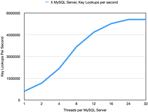
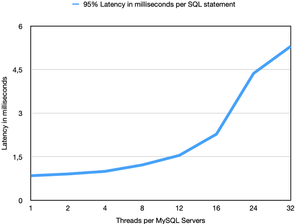
We will look at two things here, how many key lookups can be delivered per second and what is the latency of each of those batched SELECT statements.

In the image above we see how the number of key value lookups grows extremely quickly, even with only 2 threads per MySQL Server we reach beyond 1M key lookups per second. The total throughput at 32 threads is 5.56M key lookups per second.

Even more interesting is the response time of each of those SELECT statements. Remember that each of those SELECT fetch 100 rows using a primary key lookup. Using 4 threads per MySQL Server we respond within 1.0 millisecond with a throughput of 2.17M key lookups per second. At 12 threads we deliver around 4.5M key lookups with a latency around 1.5 millisecond per SELECT query. At 16 threads we deliver 5.27M key lookups at a response time of 2.28 milliseconds.

Thus as can be seen from these numbers, even using SQL, RonDB can provide astonishing key lookup performance. Obviously using C++, Java or JavaScript key-value APIs we expect to perform a lot better yet and in particular it will use much less CPU on the client side.

Research on Thread Pipelines using RonDB

 

Introduction

In my previous two blogs on this topic I first introduced the concept of automatic thread configuration and the thread model we use in RonDB. After receiving some questions on the topic I dived a bit deeper into explaining the RonDB thread model and its thread pipeline and compared it to another similar concept called batch pipelines.

Since then I read up a bit more on the research in this area with a focus on implementations in other key-value stores. Some researchers argue that a model where one handles the request immediately is superior to a model using a thread pipeline.

RonDB Software Architecture

RonDB has its roots in MySQL NDB Cluster which was developed at Ericsson in the 1990s. The execution engine in NDB has always used asynchronous programming. NDB has its roots in AXE, a telecom switch that Ericsson developed in the 1970s and still develops actually. The development model in AXE used two concepts called blocks and signals. This architecture was inherited from using a HW architecture as base for the software architecture.

The idea is that the blocks are independent units that only communicate with other blocks using signals. This is the model that all hardware is built with due to physical constraints. The reasoning in AXE was that this model is beneficial also to develop large software systems. Development of blocks can be made independent of each other as long as they handle the signalling protocols correctly.

In the 1990s CPUs were single-threaded, sometimes you had 2 CPUs on the motherboard. So a single-threaded model was good enough. When moving to a multi-threaded environment it was necessary to find a way to break up the single-threaded model into a multi-threaded model. In NDB this used two approaches, the first approach was to simply divide the blocks into execution modules. These execution modules are true to the block concept, thus they only communicate with each other through asynchronous signals. Blocks within an execution module are allowed to communicate with synchronous signals and can for optimisation purposes use direct method calls.

RonDB execution modules

In NDB the execution modules are the following:

1. Transaction Coordinator (tc)

2. Local Data Manager (ldm)

3. Main execution module (main)

4. Replication module (rep)

5. Network receive (recv)

6. Network send (send)

These execution modules are now natural to divide into threads. Each execution module can potentially be an independent thread.

However to scale RonDB to larger systems it is also necessary to split a few of those execution modules. The tc module can easily be scaled by allowing each tc module to handle its own set of transactions. This makes for a simple round-robin model to select the tc module to handle a transaction.

The ldm module can be split by partitioning the data and let each ldm module handle a subset of the data. This makes for an easy way to route the data requests to the correct ldm module.

The network receive and the network send modules can be split by partitioning on sockets. Thus each receive socket is handled by one recv module and each send socket is handled by one send module. Each recv and send module can handle multiple sockets.

Actually the send module is handled a bit using its own model where other modules can either handle the send themselves or offload it to the send module. This is not the topic for this blog, so I won’t go into more details about send modules.

One problem with this design is that partitioning the data makes perfect sense for key-value lookups that access data using a primary key. However RonDB is a key-value database with SQL capabilities, thus it is important to also perform well for more complex queries even complex join queries accessing a multitude of tables.

In the partitioned model a range scan not using the partition key has to scan all partitions. This is both beneficial and inefficient. It allows for automatic parallelisation of the range scan, but the lookup in the index tree has to be done once in each partition which increases the cost of the range scan. The solution would be to have some amount of partitioning, but to limit it.

RonDB Query threads

To alleviate this problem a new execution module was invented which is used in RonDB. This is the query execution module. This is in reality the same module as the ldm module, but it is only allowed to handle Committed Read queries. Thus all locked reads and all writes are still routed to the ldm module.

Experiment setup

Now to the point of this description. As can be seen from the above description we have a set of execution modules where each execution module can be assigned to an independent thread. This thread can participate in the thread pipeline previously described and shown in the image above.

The important thing here is that we are actually at liberty to place the execution modules into threads in any manner we like. This opens up the floor to use RonDB as a vehicle to research the benefits and deficiencies of thread pipelines.

The code used in these experiments is found in the hopsworks_2525 branch in the RonDB tree.

In this branch of RonDB it is possible to colocate the tc threads and recv execution modules. Thus each recv thread has both a tc execution module as well as a recv execution module. The assignment of the tc execution module will always be done such that the recv execution module and the tc execution module is placed in the same recv thread.

This makes it possible to create a RonDB data node where we only have separate recv threads and ldm/query threads. However I took another step and even made it possible to run RonDB with only receive threads. In this case each recv thread contains a recv, tc, ldm, and query execution module. In this case we will always select the local query module to execute the query if possible.

The above model makes it possible to experiment with the various settings.

To test this I used a micro-benchmark using variants of the Sysbench test presented here and here. The tests were executed on a P620 Lenovo workstation with a AMD Threadripper processor based on the AMD Zen 2 architecture.

To analyze the tests and to try to understand the reasons for the performance differences in the setups I used a set of perf scripts that can be found in the dbt2 benchmark tree.

The setup I am going to report here used two different setups of RonDB. The setups are not using the automated thread configuration, but rather use the ThreadConfig configuration variable that makes it possible to set up a large variety of thread configurations and experiment with those. I will add the autobench.conf used in those benchmarks at the end of the blog.

The RonDB data nodes used 4 threads that were locked to 4 CPUs using 2 CPU cores in both experiments. One experiment used 4 receive threads that try to do all processing on one thread, the second experiment used 2 receive threads that handle both the receive execution module and the tc execution module and then 1 ldm thread and 1 query thread.

We will call the set up with separated ldm and recv threads the LDM setup and the other setup will be called the Receive setup in this document.

Key-value lookups

The first experiment uses a variant where Sysbench only performs batched primary key lookups with 100 lookups in each SQL statement.

In this case the model LDM setup is able to handle 1.34M lookups per second. The Receive setup is able to handle 1.05M lookups. Thus the thread pipeline achieves almost 30% better throughput in this experiment.

Given that both experiments are executed within RonDB using exactly the same code, from the same RonDB version, it is safe to assume that the execution uses the same amount of code, the same amount of instructions are executed to perform a key-value lookup.

So what differs when looking into the CPU statistics. What is clear is that modern CPUs are very hard to analyze given that they are extremely good at parallelising tasks. 

The two things that stand out are the IPC achieved, the CPU usage and the clock frequency used. The ldm thread in the LDM setup achieves an IPC of 1.40, a frequency of 3.96 GHz and 99.8% CPU usage. The query thread has an IPC of 1.30, a frequency of 3.95 GHz and a CPU usage of 99.9%. The receive threads in the LDM setup have an IPC of 1.26, a frequency of 3.886 and a CPU usage of 66.4%.

The Receive setup threads have an IPC of 1.05, a frequency of 3.468 GHz and a 77.6% CPU usage.

Thus the performance difference comes from a combination of a higher IPC in the LDM setup, but also actually it runs at 500MHz higher clock frequency. The total CPU usage is slightly higher in the LDM setup. Those factors combined account for the 30% difference.

So trying to understand those numbers one can see that the LDM setup has a higher hit rate in the L1 data cache and slightly higher hit rate in the L1 instruction cache. There is also a slightly higher branch prediction miss rate in the Receive setup. However nothing revolutionary is seen here. The L2 miss rate is very similar in both experiments. The other difference is that the Receive setup sees a 10x higher rate iTLB misses.

The only real difference between the two cases is that the Receive setup will see more code. Thus it is expected that it will have to pay for that with more instruction cache misses, but interestingly this also triggers changes in the CPU frequency.

Thus our conclusion here is that if one can achieve a setup where the thread uses a limited amount of code to achieve its purpose, the performance will be much higher.

In principle the conclusion I do is that if we can decrease the code size we touch in a thread, this will directly affect the performance.

Using some number crunching we see that executing one key-value lookup in the ldm thread uses about 6000-7000 x86  assembler instructions. Thus the payback of decreasing the code size is almost logarithmic. So reusing the same code gives great payback in throughput of your program.

To summarize executing about 10k instructions in a single thread costs almost 30% more than

splitting up the execution in 2 threads where one thread takes care of 4k instructions and the other takes care of 6k instructions.

It isn’t expected that this gain is independent of the code size. It is likely that when the code size fits well into the L1 instruction cache, that brings about a large performance enhancement. Thus if the code size of each of threads in the thread pipeline is too big for the L1 instruction cache, it is not expected that the gain of the thread pipeline is very large. So to optimize performance one needs to keep the code size aligned with the size of the instruction cache. This means that another important factor impacting the performance is the choice of compiler flags, this choice plays together with the software architecture.

Range Scans

The next test I singled out only included range scans from Sysbench. This had two effects, first the code executed was different, in the ldm/query thread this led to even higher IPC and even higher frequency of the CPU. The IPC increased to 2.25 and the frequency increased by 2%. However another effect was that a lot more of the processing moved to the ldm/query threads, thus the receive thread was much less involved. This had the effect that the Receive setup actually had higher throughput in this case.

Outcome of tests

What we have shown with those tests is that it is beneficial from an efficiency point of view to use a thread pipeline. It increases the IPC and surprisingly also increases the frequency the CPU core operates in. This can increase the throughput up to at least 30% and even more than that in some tests executed.

At the same time the workload can cause the load to be unbalanced, this can cause some CPUs to be a bit unused. This can cause up to 30-40% loss of performance in some workloads and no loss at all and even a small gain in other workloads.

Thus the outcome is that whether or not using a thread pipeline or not is dependent on the workload. We have concluded that thread pipelines definitely provide an advantage, but also that this advantage can be wiped out by imbalances in the load on the various threads in the pipeline.

Adaptive solution

So actually when I started this exercise I expected to find out which model would work best. I wasn’t really expecting to come up with a new model as the solution. However the results made it clear that thread pipelines should be used, but that one needs to find ways of using the free CPU cycles in the LDM setup.

Given the flexibility of the query threads we have an obvious candidate for this flexibility. It is possible to execute some queries directly from the receive threads instead of passing them on to the ldm/query threads. The introduction of query threads makes it possible to be more flexible in allocating the execution of those queries.

So the conclusion is that a combination of the Receive setup and the LDM setup is the winning concept. However this introduces a new technical challenge. It is necessary to implement an adaptive algorithm that decides when to execute queries locally in the receive thread and when to execute them using the ldm/query threads.

This is in line with the development of RonDB the last couple of years. The static solutions are rarely optimal, it is often necessary to introduce adaptive algorithms that use CPU load statistics and queue size statistics for the threads in the mix.

In a sense this could be viewed as a query optimizer for key-value databases. SQL queries are usually complex and require careful selection of the execution plan for a single query. In a key-value database millions of queries per second flow through the database and by adapting the execution model to the current workload we achieve query optimisation of large flows of small simple queries.

autobench.conf

#

# Software definition

#

USE_RONDB="no"

USE_BINARY_MYSQL_TARBALL="no"

TARBALL_DIR="/home/mikael/tarballs"

MYSQL_BIN_INSTALL_DIR="/home/mikael/mysql"

BENCHMARK_TO_RUN="sysbench"

MYSQL_VERSION="rondb-gpl-21.10.0"

DBT2_VERSION="dbt2-0.37.50.17"

SYSBENCH_VERSION="sysbench-0.4.12.17"

MYSQL_BASE="8.0"

TASKSET="numactl"

#

# Storage definition

#

DATA_DIR_BASE="/home/mikael/ndb"

#

# MySQL Server definition

#

SERVER_HOST="127.0.0.1"

SERVER_PORT="3316"

ENGINE="ndb"

MYSQL_USER="root"

#

# NDB node definitions

#

NDB_EXTRA_CONNECTIONS="32"

NDB_MULTI_CONNECTION="4"

NDB_TOTAL_MEMORY="25200M"

NDB_MGMD_NODES="127.0.0.1"

NDBD_NODES="127.0.0.1"

NDB_FRAGMENT_LOG_FILE_SIZE="1G"

NDB_NO_OF_FRAGMENT_LOG_FILES="16"

NDB_SPIN_METHOD="StaticSpinning"

NDB_MAX_NO_OF_CONCURRENT_OPERATIONS="262144"

NDB_AUTOMATIC_THREAD_CONFIG="no"

NDB_THREAD_CONFIG="ldm={count=1,cpubind=0},query={count=1,cpubind=1},tc={count=0,cpubind=2},recv={count=2,cpubind=32,33},send={count=0,cpubind=35},main={count=0,cpubind=36},io={count=1,cpubind=33}"

#NDB_THREAD_CONFIG="ldm={count=0,cpubind=0},query={count=0,cpubind=3},tc={count=0,cpubind=2},recv={count=4,cpubind=0,1,32,33},send={count=0,cpubind=35},main={count=0,cpubind=36},io={count=1,cpubind=33}"

#

# Benchmark definition

#

SYSBENCH_TEST="oltp_rw"

MAX_TIME="20000"

#SB_POINT_SELECTS="0"

SB_NUM_TABLES="1"

#SB_SUM_RANGES="0"

#SB_DISTINCT_RANGES="0"

#SB_ORDER_RANGES="0"

#SB_SIMPLE_RANGES="0"

#SB_USE_IN_STATEMENT="100"

THREAD_COUNTS_TO_RUN="48"

SERVER_BIND="0"

SERVER_CPUS="8-27,40-59"

BENCHMARK_BIND="0"

BENCHMARK_CPUS="28-31,60-63"