Introduction
In my previous two blogs on this topic I first introduced the concept of automatic thread configuration and the thread model we use in RonDB. After receiving some questions on the topic I dived a bit deeper into explaining the RonDB thread model and its thread pipeline and compared it to another similar concept called batch pipelines.
Since then I read up a bit more on the research in this area with a focus on implementations in other key-value stores. Some researchers argue that a model where one handles the request immediately is superior to a model using a thread pipeline.
RonDB Software Architecture
RonDB has its roots in MySQL NDB Cluster which was developed at Ericsson in the 1990s. The execution engine in NDB has always used asynchronous programming. NDB has its roots in AXE, a telecom switch that Ericsson developed in the 1970s and still develops actually. The development model in AXE used two concepts called blocks and signals. This architecture was inherited from using a HW architecture as base for the software architecture.
The idea is that the blocks are independent units that only communicate with other blocks using signals. This is the model that all hardware is built with due to physical constraints. The reasoning in AXE was that this model is beneficial also to develop large software systems. Development of blocks can be made independent of each other as long as they handle the signalling protocols correctly.
In the 1990s CPUs were single-threaded, sometimes you had 2 CPUs on the motherboard. So a single-threaded model was good enough. When moving to a multi-threaded environment it was necessary to find a way to break up the single-threaded model into a multi-threaded model. In NDB this used two approaches, the first approach was to simply divide the blocks into execution modules. These execution modules are true to the block concept, thus they only communicate with each other through asynchronous signals. Blocks within an execution module are allowed to communicate with synchronous signals and can for optimisation purposes use direct method calls.
RonDB execution modules
In NDB the execution modules are the following:
Transaction Coordinator (tc)
Local Data Manager (ldm)
Main execution module (main)
Replication module (rep)
Network receive (recv)
Network send (send)
These execution modules are now natural to divide into threads. Each execution module can potentially be an independent thread.
However to scale RonDB to larger systems it is also necessary to split a few of those execution modules. The tc module can easily be scaled by allowing each tc module to handle its own set of transactions. This makes for a simple round-robin model to select the tc module to handle a transaction.
The ldm module can be split by partitioning the data and let each ldm module handle a subset of the data. This makes for an easy way to route the data requests to the correct ldm module.
The network receive and the network send modules can be split by partitioning on sockets. Thus each receive socket is handled by one recv module and each send socket is handled by one send module. Each recv and send module can handle multiple sockets.
Actually the send module is handled a bit using its own model where other modules can either handle the send themselves or offload it to the send module. This is not the topic for this blog, so I won’t go into more details about send modules.
One problem with this design is that partitioning the data makes perfect sense for key-value lookups that access data using a primary key. However RonDB is a key-value database with SQL capabilities, thus it is important to also perform well for more complex queries even complex join queries accessing a multitude of tables.
In the partitioned model a range scan not using the partition key has to scan all partitions. This is both beneficial and inefficient. It allows for automatic parallelisation of the range scan, but the lookup in the index tree has to be done once in each partition which increases the cost of the range scan. The solution would be to have some amount of partitioning, but to limit it.
RonDB Query threads
To alleviate this problem a new execution module was invented which is used in RonDB. This is the query execution module. This is in reality the same module as the ldm module, but it is only allowed to handle Committed Read queries. Thus all locked reads and all writes are still routed to the ldm module.

Experiment setup
Now to the point of this description. As can be seen from the above description we have a set of execution modules where each execution module can be assigned to an independent thread. This thread can participate in the thread pipeline previously described and shown in the image above.
The important thing here is that we are actually at liberty to place the execution modules into threads in any manner we like. This opens up the floor to use RonDB as a vehicle to research the benefits and deficiencies of thread pipelines.
The code used in these experiments is found in the hopsworks_2525 branch in the RonDB tree.
In this branch of RonDB it is possible to colocate the tc threads and recv execution modules. Thus each recv thread has both a tc execution module as well as a recv execution module. The assignment of the tc execution module will always be done such that the recv execution module and the tc execution module is placed in the same recv thread.
This makes it possible to create a RonDB data node where we only have separate recv threads and ldm/query threads. However I took another step and even made it possible to run RonDB with only receive threads. In this case each recv thread contains a recv, tc, ldm, and query execution module. In this case we will always select the local query module to execute the query if possible.
The above model makes it possible to experiment with the various settings.
To test this I used a micro-benchmark using variants of the Sysbench test presented here and here. The tests were executed on a P620 Lenovo workstation with a AMD Threadripper processor based on the AMD Zen 2 architecture.
To analyze the tests and to try to understand the reasons for the performance differences in the setups I used a set of perf scripts that can be found in the dbt2 benchmark tree.
The setup I am going to report here used two different setups of RonDB. The setups are not using the automated thread configuration, but rather use the ThreadConfig configuration variable that makes it possible to set up a large variety of thread configurations and experiment with those. I will add the autobench.conf used in those benchmarks at the end of the blog.
The RonDB data nodes used 4 threads that were locked to 4 CPUs using 2 CPU cores in both experiments. One experiment used 4 receive threads that try to do all processing on one thread, the second experiment used 2 receive threads that handle both the receive execution module and the tc execution module and then 1 ldm thread and 1 query thread.
We will call the set up with separated ldm and recv threads the LDM setup and the other setup will be called the Receive setup in this document.
Key-value lookups
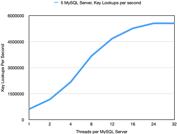
The first experiment uses a variant where Sysbench only performs batched primary key lookups with 100 lookups in each SQL statement.
In this case the model LDM setup is able to handle 1.34M lookups per second. The Receive setup is able to handle 1.05M lookups. Thus the thread pipeline achieves almost 30% better throughput in this experiment.
Given that both experiments are executed within RonDB using exactly the same code, from the same RonDB version, it is safe to assume that the execution uses the same amount of code, the same amount of instructions are executed to perform a key-value lookup.
So what differs when looking into the CPU statistics. What is clear is that modern CPUs are very hard to analyze given that they are extremely good at parallelising tasks.
The two things that stand out are the IPC achieved, the CPU usage and the clock frequency used. The ldm thread in the LDM setup achieves an IPC of 1.40, a frequency of 3.96 GHz and 99.8% CPU usage. The query thread has an IPC of 1.30, a frequency of 3.95 GHz and a CPU usage of 99.9%. The receive threads in the LDM setup have an IPC of 1.26, a frequency of 3.886 and a CPU usage of 66.4%.
The Receive setup threads have an IPC of 1.05, a frequency of 3.468 GHz and a 77.6% CPU usage.
Thus the performance difference comes from a combination of a higher IPC in the LDM setup, but also actually it runs at 500MHz higher clock frequency. The total CPU usage is slightly higher in the LDM setup. Those factors combined account for the 30% difference.
So trying to understand those numbers one can see that the LDM setup has a higher hit rate in the L1 data cache and slightly higher hit rate in the L1 instruction cache. There is also a slightly higher branch prediction miss rate in the Receive setup. However nothing revolutionary is seen here. The L2 miss rate is very similar in both experiments. The other difference is that the Receive setup sees a 10x higher rate iTLB misses.
The only real difference between the two cases is that the Receive setup will see more code. Thus it is expected that it will have to pay for that with more instruction cache misses, but interestingly this also triggers changes in the CPU frequency.
Thus our conclusion here is that if one can achieve a setup where the thread uses a limited amount of code to achieve its purpose, the performance will be much higher.
In principle the conclusion I do is that if we can decrease the code size we touch in a thread, this will directly affect the performance.
Using some number crunching we see that executing one key-value lookup in the ldm thread uses about 6000-7000 x86 assembler instructions. Thus the payback of decreasing the code size is almost logarithmic. So reusing the same code gives great payback in throughput of your program.
To summarize executing about 10k instructions in a single thread costs almost 30% more than
splitting up the execution in 2 threads where one thread takes care of 4k instructions and the other takes care of 6k instructions.
It isn’t expected that this gain is independent of the code size. It is likely that when the code size fits well into the L1 instruction cache, that brings about a large performance enhancement. Thus if the code size of each of threads in the thread pipeline is too big for the L1 instruction cache, it is not expected that the gain of the thread pipeline is very large. So to optimize performance one needs to keep the code size aligned with the size of the instruction cache. This means that another important factor impacting the performance is the choice of compiler flags, this choice plays together with the software architecture.
Range Scans
The next test I singled out only included range scans from Sysbench. This had two effects, first the code executed was different, in the ldm/query thread this led to even higher IPC and even higher frequency of the CPU. The IPC increased to 2.25 and the frequency increased by 2%. However another effect was that a lot more of the processing moved to the ldm/query threads, thus the receive thread was much less involved. This had the effect that the Receive setup actually had higher throughput in this case.
Outcome of tests
What we have shown with those tests is that it is beneficial from an efficiency point of view to use a thread pipeline. It increases the IPC and surprisingly also increases the frequency the CPU core operates in. This can increase the throughput up to at least 30% and even more than that in some tests executed.
At the same time the workload can cause the load to be unbalanced, this can cause some CPUs to be a bit unused. This can cause up to 30-40% loss of performance in some workloads and no loss at all and even a small gain in other workloads.
Thus the outcome is that whether or not using a thread pipeline or not is dependent on the workload. We have concluded that thread pipelines definitely provide an advantage, but also that this advantage can be wiped out by imbalances in the load on the various threads in the pipeline.
Adaptive solution
So actually when I started this exercise I expected to find out which model would work best. I wasn’t really expecting to come up with a new model as the solution. However the results made it clear that thread pipelines should be used, but that one needs to find ways of using the free CPU cycles in the LDM setup.
Given the flexibility of the query threads we have an obvious candidate for this flexibility. It is possible to execute some queries directly from the receive threads instead of passing them on to the ldm/query threads. The introduction of query threads makes it possible to be more flexible in allocating the execution of those queries.
So the conclusion is that a combination of the Receive setup and the LDM setup is the winning concept. However this introduces a new technical challenge. It is necessary to implement an adaptive algorithm that decides when to execute queries locally in the receive thread and when to execute them using the ldm/query threads.
This is in line with the development of RonDB the last couple of years. The static solutions are rarely optimal, it is often necessary to introduce adaptive algorithms that use CPU load statistics and queue size statistics for the threads in the mix.
In a sense this could be viewed as a query optimizer for key-value databases. SQL queries are usually complex and require careful selection of the execution plan for a single query. In a key-value database millions of queries per second flow through the database and by adapting the execution model to the current workload we achieve query optimisation of large flows of small simple queries.
autobench.conf
#
# Software definition
#
USE_RONDB="no"
USE_BINARY_MYSQL_TARBALL="no"
TARBALL_DIR="/home/mikael/tarballs"
MYSQL_BIN_INSTALL_DIR="/home/mikael/mysql"
BENCHMARK_TO_RUN="sysbench"
MYSQL_VERSION="rondb-gpl-21.10.0"
DBT2_VERSION="dbt2-0.37.50.17"
SYSBENCH_VERSION="sysbench-0.4.12.17"
MYSQL_BASE="8.0"
TASKSET="numactl"
#
# Storage definition
#
DATA_DIR_BASE="/home/mikael/ndb"
#
# MySQL Server definition
#
SERVER_HOST="127.0.0.1"
SERVER_PORT="3316"
ENGINE="ndb"
MYSQL_USER="root"
#
# NDB node definitions
#
NDB_EXTRA_CONNECTIONS="32"
NDB_MULTI_CONNECTION="4"
NDB_TOTAL_MEMORY="25200M"
NDB_MGMD_NODES="127.0.0.1"
NDBD_NODES="127.0.0.1"
NDB_FRAGMENT_LOG_FILE_SIZE="1G"
NDB_NO_OF_FRAGMENT_LOG_FILES="16"
NDB_SPIN_METHOD="StaticSpinning"
NDB_MAX_NO_OF_CONCURRENT_OPERATIONS="262144"
NDB_AUTOMATIC_THREAD_CONFIG="no"
NDB_THREAD_CONFIG="ldm={count=1,cpubind=0},query={count=1,cpubind=1},tc={count=0,cpubind=2},recv={count=2,cpubind=32,33},send={count=0,cpubind=35},main={count=0,cpubind=36},io={count=1,cpubind=33}"
#NDB_THREAD_CONFIG="ldm={count=0,cpubind=0},query={count=0,cpubind=3},tc={count=0,cpubind=2},recv={count=4,cpubind=0,1,32,33},send={count=0,cpubind=35},main={count=0,cpubind=36},io={count=1,cpubind=33}"
#
# Benchmark definition
#
SYSBENCH_TEST="oltp_rw"
MAX_TIME="20000"
#SB_POINT_SELECTS="0"
SB_NUM_TABLES="1"
#SB_SUM_RANGES="0"
#SB_DISTINCT_RANGES="0"
#SB_ORDER_RANGES="0"
#SB_SIMPLE_RANGES="0"
#SB_USE_IN_STATEMENT="100"
THREAD_COUNTS_TO_RUN="48"
SERVER_BIND="0"
SERVER_CPUS="8-27,40-59"
BENCHMARK_BIND="0"
BENCHMARK_CPUS="28-31,60-63"