Showing posts with label key-value store. Show all posts

Monday, May 27, 2024

875X improvement from RonDB 21.04.17 to 22.10.4

At Hopsworks we are working on ensuring that the online feature store will be able to perform complex join operations in real-time. This means that queries that could use data from multiple tables can be easily integrated into machine learning applications.

Today most feature stores use key-value stores like Redis and DynamoDB. These systems have no capability to issue complex join queries, if this is required the feature store will have to write complex code to handle this and this is likely to involve multiple roundtrips and thus cause unwanted latency.

Hopsworks feature store uses RonDB as its online feature store. RonDB can handle any SQL operations that MySQL can handle. Actually RonDB has even support for parallelising the join queries and pushing the filtering and joining down to the RonDB data nodes where data resides.

This means that users of the Hopsworks feature store can integrate more features from multiple feature groups in online inferencing requests. This means that things credit fraud detection can be made much more intelligent by taking more features into account in the inferencing requests.

This means that performance of real-time join queries becomes more important in RonDB. To evaluate how RonDB develops in this are I ran a set of tests using TPC-H queries from DBT3 against RonDB 21.04.17 and RonDB 22.10.4 (not released yet). I also ran tests against MySQL 8.0.35 (RonDB 22.10.4 is based on MySQL 8.0.35 with loads of added RonDB features).

The results were interesting, the improvement in Q20 was the highest I have seen in my career. The performance improved from 70 seconds to 80 milliseconds, thus an 875x speedup or 87500% improvement. Q2 had a 360x improvement. So RonDB 22.10.4 is much better equipped for more complex queries compared to RonDB 21.04. MySQL 8.0.35 had similar performance to RonDB 22.10.4 with an average of around 20% slower, this is mostly due to performance improvements in RonDB, not algorithmic changes.

When using complex queries the query optimiser tries to find an optimal plan, sometimes however better plans are available and one can add hints in the SQL query to ensure a better plan is used.

The RonDB team isn't satisfied with this however, we have realised that evaluating aggregation is also very important when the online feature store stores a time window of certain features. This means that RonDB can compute aggregate dynamically and thus provide more accurate predictions.

Early tests of some simple single table queries showed an improvement of 4-5x and we expect we will be able to get to 10-20x improvements in quite a few queries of this sort.

Thursday, October 26, 2023

Results on comparing new Intel/AMD VMs with older VM types using RonDB

 In Hopsworks cloud offering for GCP one can select a fairly large variety of VM types. I am currently working on extending this list to also include the latest generation of VM types. This blog will focus on the impact of those new VM types for benchmarks using RonDB.

The newer VM types is the c3d-serie that uses AMD EPYC CPUs of the 4th generation and the c3-series which contains VMs using the Intel Saphire Rapid CPUs. Also AWS has introduced similar new VM types, but this blog discuss tests performed on VMs in GCP.

The older VM types we compared with for the MySQL Servers was the n2-standard-16 VM type. This VM uses an Intel Cascade Lake Xeon processor. This represents the second generation Intel Xeon chips whereas Intel Saphire Rapid represents the 4th generation Intel Xeon.

The RonDB data nodes used the e2-highmem-16 as the baseline for comparison. This VM types uses either an Intel Xeon of the second generation or an AMD EPYC of the second generation.

The benchmark used was Sysbench OLTP RW based on version 0.4.12.19 which is included in the RonDB tarball and is setup in the API nodes automatically by our cloud offering. This makes it extremely easy to replicate the benchmarks. We use Consul as a load balancer, so the benchmark process is setup to a single host onlinefs.mysql.service.consul. In reality this address maps to the number of MySQL Servers in the RonDB cluster. We used 3 MySQL Servers in the tests. The setup used 2 RonDB data nodes in one node group.

Thus in the Hopsworks cloud we get a load balanced RonDB Data Service as part of the infrastructure of the Hopsworks Feature Store.

We first executed the benchmark using the old VM types to get a baseline. The next step was to upgrade the RonDB MySQL Servers to use c3d-highmem-16. Thus the same amount of memory and number of CPUs as in n2-standard-16 but upgraded from Intel 2nd generation to AMD 4th generation.

This impacted the throughput mainly. The baseline experiment executed 9000 TPS and was limited by the CPUs in the MySQL Servers (they used 1550% of the 1600% available). The c3d-highmem-16 delivered 11400 TPS but only using 1000% of the available 1600%. Thus the throughput per CPU increased by around 100%. In this execution the bottleneck of the benchmark was the RonDB data nodes.

The benchmark API node was consistently a n2-standard-48 VM. This meant that most communication went from API VM of old type, to MySQL Server of new type, to RonDB data node VM of old type. Thus in all communication an old VM type was involved. The network latency was the same in this experiment as in the baseline experiment.

The change from one VM type was using the Reconfiguration support RonDB have in its Cloud offering. This change is an online operation where the cluster remains operational and the new MySQL Servers are included in the Consul setup as soon as they have started up. Only when nodes are stopped could temporary errors happen that can be handled with a simple retry logic.

Next we changed also the VM type of the RonDB data nodes to be c3d-highmem-16 using the same online reconfiguration as for the MySQL Servers.

What we quickly noted in this setup was that the latency per transaction was cut in half. Thus performance using a single thread decreased to less than half. Thus it is clear that communication between 2 VMs of the new type have more than 100% improvements on network latency. The throughput now increased to 17800 TPS and the bottleneck was now in the MySQL Servers. Thus throughput improvement is almost 98% and network latency improved by more than 100%.

When reading the announcement of the C3 machine series and the description of the C3D machine series, it is clear that the new IPU (Infrastructure Processing Unit) that takes care of offloading networking is a major reason for this improved network latency.

Analysing the Sysbench transaction in this setup there will be around 100 network messages, most of them in serial order. Still the latency of a transaction execution is no more than 6 milliseconds to execute the 20 SQL queries involved in the OLTP RW transaction. Thus a medium of 60 microsecond per message and this includes the time to also execute the RonDB Data node code and the RonDB MySQL Server code.

Next step was to again change MySQL Server VMs. This time we changed to c3-highmem-22. Unfortunately the VM type c3-highmem-16 didn't exist. So the comparison isn't perfect, but at least it gives a good estimate of the improvements in Intel's 4th generation CPUs.

The network latency was the same for Intel and AMD 4th generation VM types. The throughput increased by around 40% up to around 24000 TPS. Since the number of CPUs increased by around 40% as well, it seems that c3-serie and c3d-serie is very similar in handling throughput when used in RonDB MySQL Servers.

To test the throughput of those new VMs we ran the test using c3-highmem-8 and c3d-highmem-8 VM types as RonDB Data node VMs. The performance of those two VM types was almost indistinguishable, to the point where I started wondering if they were the same CPUs. Throughput was half the throughput of the 16 VCPU VMs.

The main conclusion of these tests is that upgrading from 2nd generation x86 CPUs to 4th generation x86 CPUs in the GCP cloud provides a 100% improvement in throughput and a similar improvement of the network latency.

The price of those VMs is higher, but substantially less than 100%. So it makes a lot of sense to start using those new VM types for new applications.

The tests were performed using the RonDB version 21.04.15. We are about to release a new LTS version of RonDB, version 22.10.1. There will be a more thorough benchmark report when this is released.

Monday, January 31, 2022

RonDB receives ARM64 support and large transaction support

 RonDB is the base platform for all applications in Hopsworks. Hopsworks is a machine learning platform featuring a Feature Store that can be used in online applications as well as offline applications.

This means that RonDB development is driven towards ensuring that operating RonDB in this environment is the best possible.

RonDB is designed for millions of small transactions reading and writing data. However occasionally applications perform rather large transactions. Previous versions of RonDB had some weaknesses in this area. The new versions of RonDB now supports also large transactions although the focus is still on many smaller transactions.

Designing this new support of large transactions required a fairly large development effort. To do this in a stable release is a challenge, therefore it was decided to combine this effort with a heavy testing period focused on fixing bugs.

This effort has been focused on achieving three objectives. First to stabilise the new RonDB 21.04 releases which is the stable release of RonDB. Second, to stabilise the next RonDB release at the same level as RonDB 21.04. Third, we also wanted the same level of support for ARM64 machines.

We are now proud to release RonDB 21.04.3, a new stable release of RonDB that supports much larger transactions. Since the release of RonDB 21.04.1 in July 2021 we have fixed more than 50 bugs in RonDB and we are very satisfied with the stability also on ARM64 machines.

The original plan was to release the next version of RonDB in October 2021, however we didn't want to release a new version with any less stability than the RonDB 21.04 release. Thus instead we release this new version of RonDB now, RonDB 22.01.0.

ARM64 support covers both RonDB 21.04.3 and RonDB 22.01.0. RonDB is now also supported on both Linux and Mac OS X and on Windows it is supported using WSL 2 (Linux on Windows) on Windows 11. We have extensively tested RonDB on the following platforms:

  1. Mac OS X 11.6 x86_64
  2. Mac OS X 12.2 ARM64
  3. Windows WSL 2 Ubuntu x86_64
  4. Ubuntu 21.04 x86_64
  5. Oracle Linux 8 Cloud Developer version ARM64

It is used in production on AWS and Azure and has been extensively tested also on GCP and Oracle Cloud.

As part of the new RonDB release we have also updated the documentation of RonDB at docs.rondb.com. Among other things it contains a new section on Contributing to RonDB that shows how you can build, test and develop extensions to RonDB. In the documentation you will also find an extensive list of the improvements made in the two new RonDB releases.

ARM64 support is still in beta phase, our plan is to make it available for production use in Q2 2022. There are no known bugs, but we want to give it a bit more time before we assign it to production workloads. This includes adding more test machines and also performing benchmarks on ARM64 VMs.

Our experience with ARM64 machines so far says that it is fairly stable, but it isn't yet at the same level as x86, it is possible to find bugs in the compilers, the support around it is however maturing very quickly and not surprising the support on Mac OS X is here leading the way since Mac OS X has fully committed its future on ARM. We have also great help of participating in the OCI ARM Accelerator program providing access to ARM VMs in the Oracle Cloud making it possible to test on Oracle Linux using ARM with both small and large VMs.

RonDB 22.01.0 comes with a set of new features:

  1. Now possible to scale reads using locks onto more threads
  2. Improved placement of primary replicas to enable
  3. All major memory areas now managed by global memory manager
  4. Even more flexibility in thread configurations
  5. Removing a scalability hog in index statistics handling
  6. Merged with MySQL Cluster 8.0.28

You can either download RonDB tarballs from https://github.com/logicalclocks/rondb or from https://repo.hops.works/master, for exact links to the various versions of the binary tarballs see Release Notes on each version.

Wednesday, May 19, 2021

5.5M Key Lookups per second on 16 VCPU VMs

 As introduced in a previous blog RonDB enables us to easily execute benchmarks on RonDB using the Sysbench benchmark.


In this blog I will present some results where the RonDB cluster had 2 data nodes, each using a r5.4xlarge VM in AWS that has 16 VCPUs and 128 GB memory. The Sysbench test uses SQL to access RonDB.


In this particular test case we wanted to test the Key-Lookup performance using SQL. Key-Lookup performance is essential in the RonDB use case as an online Feature Store in Hopsworks.


In this case we use the following settings in the Sysbench configuration file (see RonDB documentation for more details on how to set up those tests):


SB_USE_IN_STATEMENT=”100”

SYSBENCH_TEST=”oltp_ro”

SB_SIMPLE_RANGES=”0”

SB_ORDER_RANGES=”0”

SB_SUM_RANGES=”0”

SB_DISTINCT_RANGES=”0”


These settings means that each transaction has 10 SQL queries, each of those queries fetch 100 rows using a primary key lookup. Thus each transaction performs 1000 key lookups.


We will look at two things here, how many key lookups can be delivered per second and what is the latency of each of those batched SELECT statements.


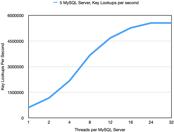
In the image above we see how the number of key value lookups grows extremely quickly, even with only 2 threads per MySQL Server we reach beyond 1M key lookups per second. The total throughput at 32 threads is 5.56M key lookups per second.


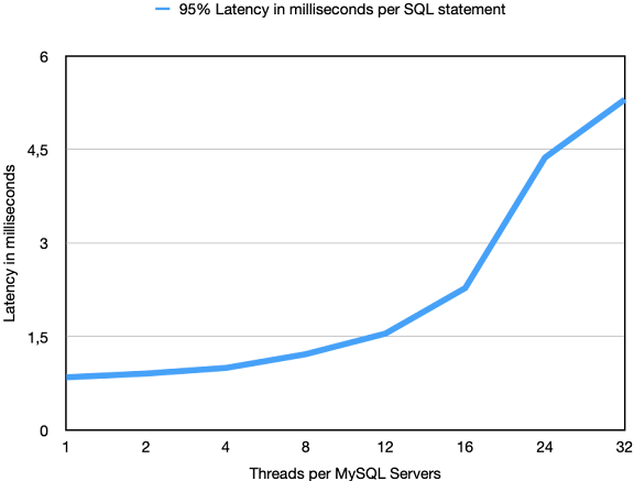
Even more interesting is the response time of each of those SELECT statements. Remember that each of those SELECT fetch 100 rows using a primary key lookup. Using 4 threads per MySQL Server we respond within 1.0 millisecond with a throughput of 2.17M key lookups per second. At 12 threads we deliver around 4.5M key lookups with a latency around 1.5 millisecond per SELECT query. At 16 threads we deliver 5.27M key lookups at a response time of 2.28 milliseconds.


Thus as can be seen from these numbers, even using SQL, RonDB can provide astonishing key lookup performance. Obviously using C++, Java or JavaScript key-value APIs we expect to perform a lot better yet and in particular it will use much less CPU on the client side.


Monday, May 10, 2021

Research on Thread Pipelines using RonDB


Introduction

In my previous two blogs on this topic I first introduced the concept of automatic thread configuration and the thread model we use in RonDB. After receiving some questions on the topic I dived a bit deeper into explaining the RonDB thread model and its thread pipeline and compared it to another similar concept called batch pipelines.


Since then I read up a bit more on the research in this area with a focus on implementations in other key-value stores. Some researchers argue that a model where one handles the request immediately is superior to a model using a thread pipeline.

RonDB Software Architecture

RonDB has its roots in MySQL NDB Cluster which was developed at Ericsson in the 1990s. The execution engine in NDB has always used asynchronous programming. NDB has its roots in AXE, a telecom switch that Ericsson developed in the 1970s and still develops actually. The development model in AXE used two concepts called blocks and signals. This architecture was inherited from using a HW architecture as base for the software architecture.


The idea is that the blocks are independent units that only communicate with other blocks using signals. This is the model that all hardware is built with due to physical constraints. The reasoning in AXE was that this model is beneficial also to develop large software systems. Development of blocks can be made independent of each other as long as they handle the signalling protocols correctly.


In the 1990s CPUs were single-threaded, sometimes you had 2 CPUs on the motherboard. So a single-threaded model was good enough. When moving to a multi-threaded environment it was necessary to find a way to break up the single-threaded model into a multi-threaded model. In NDB this used two approaches, the first approach was to simply divide the blocks into execution modules. These execution modules are true to the block concept, thus they only communicate with each other through asynchronous signals. Blocks within an execution module are allowed to communicate with synchronous signals and can for optimisation purposes use direct method calls.

RonDB execution modules


In NDB the execution modules are the following:

  1. Transaction Coordinator (tc)

  2. Local Data Manager (ldm)

  3. Main execution module (main)

  4. Replication module (rep)

  5. Network receive (recv)

  6. Network send (send)


These execution modules are now natural to divide into threads. Each execution module can potentially be an independent thread.


However to scale RonDB to larger systems it is also necessary to split a few of those execution modules. The tc module can easily be scaled by allowing each tc module to handle its own set of transactions. This makes for a simple round-robin model to select the tc module to handle a transaction.


The ldm module can be split by partitioning the data and let each ldm module handle a subset of the data. This makes for an easy way to route the data requests to the correct ldm module.


The network receive and the network send modules can be split by partitioning on sockets. Thus each receive socket is handled by one recv module and each send socket is handled by one send module. Each recv and send module can handle multiple sockets.


Actually the send module is handled a bit using its own model where other modules can either handle the send themselves or offload it to the send module. This is not the topic for this blog, so I won’t go into more details about send modules.


One problem with this design is that partitioning the data makes perfect sense for key-value lookups that access data using a primary key. However RonDB is a key-value database with SQL capabilities, thus it is important to also perform well for more complex queries even complex join queries accessing a multitude of tables.


In the partitioned model a range scan not using the partition key has to scan all partitions. This is both beneficial and inefficient. It allows for automatic parallelisation of the range scan, but the lookup in the index tree has to be done once in each partition which increases the cost of the range scan. The solution would be to have some amount of partitioning, but to limit it.

RonDB Query threads


To alleviate this problem a new execution module was invented which is used in RonDB. This is the query execution module. This is in reality the same module as the ldm module, but it is only allowed to handle Committed Read queries. Thus all locked reads and all writes are still routed to the ldm module.

Experiment setup

Now to the point of this description. As can be seen from the above description we have a set of execution modules where each execution module can be assigned to an independent thread. This thread can participate in the thread pipeline previously described and shown in the image above.


The important thing here is that we are actually at liberty to place the execution modules into threads in any manner we like. This opens up the floor to use RonDB as a vehicle to research the benefits and deficiencies of thread pipelines.


The code used in these experiments is found in the hopsworks_2525 branch in the RonDB tree.


In this branch of RonDB it is possible to colocate the tc threads and recv execution modules. Thus each recv thread has both a tc execution module as well as a recv execution module. The assignment of the tc execution module will always be done such that the recv execution module and the tc execution module is placed in the same recv thread.


This makes it possible to create a RonDB data node where we only have separate recv threads and ldm/query threads. However I took another step and even made it possible to run RonDB with only receive threads. In this case each recv thread contains a recv, tc, ldm, and query execution module. In this case we will always select the local query module to execute the query if possible.


The above model makes it possible to experiment with the various settings.


To test this I used a micro-benchmark using variants of the Sysbench test presented here and here. The tests were executed on a P620 Lenovo workstation with a AMD Threadripper processor based on the AMD Zen 2 architecture.


To analyze the tests and to try to understand the reasons for the performance differences in the setups I used a set of perf scripts that can be found in the dbt2 benchmark tree.


The setup I am going to report here used two different setups of RonDB. The setups are not using the automated thread configuration, but rather use the ThreadConfig configuration variable that makes it possible to set up a large variety of thread configurations and experiment with those. I will add the autobench.conf used in those benchmarks at the end of the blog.


The RonDB data nodes used 4 threads that were locked to 4 CPUs using 2 CPU cores in both experiments. One experiment used 4 receive threads that try to do all processing on one thread, the second experiment used 2 receive threads that handle both the receive execution module and the tc execution module and then 1 ldm thread and 1 query thread.


We will call the set up with separated ldm and recv threads the LDM setup and the other setup will be called the Receive setup in this document.

Key-value lookups

The first experiment uses a variant where Sysbench only performs batched primary key lookups with 100 lookups in each SQL statement.


In this case the model LDM setup is able to handle 1.34M lookups per second. The Receive setup is able to handle 1.05M lookups. Thus the thread pipeline achieves almost 30% better throughput in this experiment.


Given that both experiments are executed within RonDB using exactly the same code, from the same RonDB version, it is safe to assume that the execution uses the same amount of code, the same amount of instructions are executed to perform a key-value lookup.


So what differs when looking into the CPU statistics. What is clear is that modern CPUs are very hard to analyze given that they are extremely good at parallelising tasks. 


The two things that stand out are the IPC achieved, the CPU usage and the clock frequency used. The ldm thread in the LDM setup achieves an IPC of 1.40, a frequency of 3.96 GHz and 99.8% CPU usage. The query thread has an IPC of 1.30, a frequency of 3.95 GHz and a CPU usage of 99.9%. The receive threads in the LDM setup have an IPC of 1.26, a frequency of 3.886 and a CPU usage of 66.4%.


The Receive setup threads have an IPC of 1.05, a frequency of 3.468 GHz and a 77.6% CPU usage.


Thus the performance difference comes from a combination of a higher IPC in the LDM setup, but also actually it runs at 500MHz higher clock frequency. The total CPU usage is slightly higher in the LDM setup. Those factors combined account for the 30% difference.


So trying to understand those numbers one can see that the LDM setup has a higher hit rate in the L1 data cache and slightly higher hit rate in the L1 instruction cache. There is also a slightly higher branch prediction miss rate in the Receive setup. However nothing revolutionary is seen here. The L2 miss rate is very similar in both experiments. The other difference is that the Receive setup sees a 10x higher rate iTLB misses.


The only real difference between the two cases is that the Receive setup will see more code. Thus it is expected that it will have to pay for that with more instruction cache misses, but interestingly this also triggers changes in the CPU frequency.


Thus our conclusion here is that if one can achieve a setup where the thread uses a limited amount of code to achieve its purpose, the performance will be much higher.


In principle the conclusion I do is that if we can decrease the code size we touch in a thread, this will directly affect the performance.


Using some number crunching we see that executing one key-value lookup in the ldm thread uses about 6000-7000 x86  assembler instructions. Thus the payback of decreasing the code size is almost logarithmic. So reusing the same code gives great payback in throughput of your program.


To summarize executing about 10k instructions in a single thread costs almost 30% more than

splitting up the execution in 2 threads where one thread takes care of 4k instructions and the other takes care of 6k instructions.


It isn’t expected that this gain is independent of the code size. It is likely that when the code size fits well into the L1 instruction cache, that brings about a large performance enhancement. Thus if the code size of each of threads in the thread pipeline is too big for the L1 instruction cache, it is not expected that the gain of the thread pipeline is very large. So to optimize performance one needs to keep the code size aligned with the size of the instruction cache. This means that another important factor impacting the performance is the choice of compiler flags, this choice plays together with the software architecture.

Range Scans

The next test I singled out only included range scans from Sysbench. This had two effects, first the code executed was different, in the ldm/query thread this led to even higher IPC and even higher frequency of the CPU. The IPC increased to 2.25 and the frequency increased by 2%. However another effect was that a lot more of the processing moved to the ldm/query threads, thus the receive thread was much less involved. This had the effect that the Receive setup actually had higher throughput in this case.

Outcome of tests

What we have shown with those tests is that it is beneficial from an efficiency point of view to use a thread pipeline. It increases the IPC and surprisingly also increases the frequency the CPU core operates in. This can increase the throughput up to at least 30% and even more than that in some tests executed.


At the same time the workload can cause the load to be unbalanced, this can cause some CPUs to be a bit unused. This can cause up to 30-40% loss of performance in some workloads and no loss at all and even a small gain in other workloads.


Thus the outcome is that whether or not using a thread pipeline or not is dependent on the workload. We have concluded that thread pipelines definitely provide an advantage, but also that this advantage can be wiped out by imbalances in the load on the various threads in the pipeline.

Adaptive solution

So actually when I started this exercise I expected to find out which model would work best. I wasn’t really expecting to come up with a new model as the solution. However the results made it clear that thread pipelines should be used, but that one needs to find ways of using the free CPU cycles in the LDM setup.


Given the flexibility of the query threads we have an obvious candidate for this flexibility. It is possible to execute some queries directly from the receive threads instead of passing them on to the ldm/query threads. The introduction of query threads makes it possible to be more flexible in allocating the execution of those queries.


So the conclusion is that a combination of the Receive setup and the LDM setup is the winning concept. However this introduces a new technical challenge. It is necessary to implement an adaptive algorithm that decides when to execute queries locally in the receive thread and when to execute them using the ldm/query threads.


This is in line with the development of RonDB the last couple of years. The static solutions are rarely optimal, it is often necessary to introduce adaptive algorithms that use CPU load statistics and queue size statistics for the threads in the mix.


In a sense this could be viewed as a query optimizer for key-value databases. SQL queries are usually complex and require careful selection of the execution plan for a single query. In a key-value database millions of queries per second flow through the database and by adapting the execution model to the current workload we achieve query optimisation of large flows of small simple queries.


autobench.conf

#

# Software definition

#

USE_RONDB="no"

USE_BINARY_MYSQL_TARBALL="no"

TARBALL_DIR="/home/mikael/tarballs"

MYSQL_BIN_INSTALL_DIR="/home/mikael/mysql"

BENCHMARK_TO_RUN="sysbench"

MYSQL_VERSION="rondb-gpl-21.10.0"

DBT2_VERSION="dbt2-0.37.50.17"

SYSBENCH_VERSION="sysbench-0.4.12.17"

MYSQL_BASE="8.0"

TASKSET="numactl"

#

# Storage definition

#

DATA_DIR_BASE="/home/mikael/ndb"

#

# MySQL Server definition

#

SERVER_HOST="127.0.0.1"

SERVER_PORT="3316"

ENGINE="ndb"

MYSQL_USER="root"

#

# NDB node definitions

#

NDB_EXTRA_CONNECTIONS="32"

NDB_MULTI_CONNECTION="4"

NDB_TOTAL_MEMORY="25200M"

NDB_MGMD_NODES="127.0.0.1"

NDBD_NODES="127.0.0.1"

NDB_FRAGMENT_LOG_FILE_SIZE="1G"

NDB_NO_OF_FRAGMENT_LOG_FILES="16"

NDB_SPIN_METHOD="StaticSpinning"

NDB_MAX_NO_OF_CONCURRENT_OPERATIONS="262144"

NDB_AUTOMATIC_THREAD_CONFIG="no"

NDB_THREAD_CONFIG="ldm={count=1,cpubind=0},query={count=1,cpubind=1},tc={count=0,cpubind=2},recv={count=2,cpubind=32,33},send={count=0,cpubind=35},main={count=0,cpubind=36},io={count=1,cpubind=33}"

#NDB_THREAD_CONFIG="ldm={count=0,cpubind=0},query={count=0,cpubind=3},tc={count=0,cpubind=2},recv={count=4,cpubind=0,1,32,33},send={count=0,cpubind=35},main={count=0,cpubind=36},io={count=1,cpubind=33}"

#

# Benchmark definition

#

SYSBENCH_TEST="oltp_rw"

MAX_TIME="20000"

#SB_POINT_SELECTS="0"

SB_NUM_TABLES="1"

#SB_SUM_RANGES="0"

#SB_DISTINCT_RANGES="0"

#SB_ORDER_RANGES="0"

#SB_SIMPLE_RANGES="0"

#SB_USE_IN_STATEMENT="100"

THREAD_COUNTS_TO_RUN="48"

SERVER_BIND="0"

SERVER_CPUS="8-27,40-59"

BENCHMARK_BIND="0"

BENCHMARK_CPUS="28-31,60-63"


Wednesday, May 05, 2021

Sysbench evaluation of RonDB


Introduction

Sysbench is a tool to benchmark to test open source databases. We have integrated Sysbench into the RonDB installation. This makes it extremely easy to run benchmarks with RonDB. This paper will describe the use of these benchmarks in RonDB. These benchmarks were executed with 1 cluster connection per MySQL Server. This limited the scalability per MySQL Server to about 12 VCPUs. Since we executed those benchmarks we have increased the number of cluster connections per MySQL Server to 4 providing scalability to at least 32 VCPUs per MySQL Server.


As preparation to run those benchmarks we have created a RonDB cluster using the Hopsworks framework that is currently used to create RonDB clusters. In these tests all MySQL Servers are using the c5.4xlarge VM instances in AWS (16 VCPUs with 32 GB memory). We have a RonDB management server using the t3a.medium VM instance type. We have tested using two different RonDB clusters, both have 2 data nodes. The first test is using the r5.4xlarge instance type (16 VCPUs and 128 GB memory) and the second test uses the r5n.8xlarge (32 VCPUs and 256 GB memory). It was necessary to use r5n class since we needed more than 10Gbit/second network bandwidth for the OLTP RW test with 32 VCPUs on data nodes.


In the RonDB documentation you can find more details how to set up your own RonDB cluster in either our managed version (currently supporting AWS) or using our open source shell scripts to set up a cluster (currently supporting GCP and Azure). RonDB is a new distribution of MySQL NDB Cluster. All experiments in this blog was performed using RonDB 21.04.0.


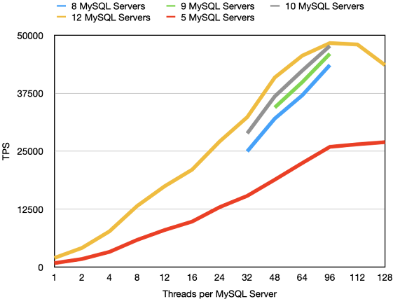
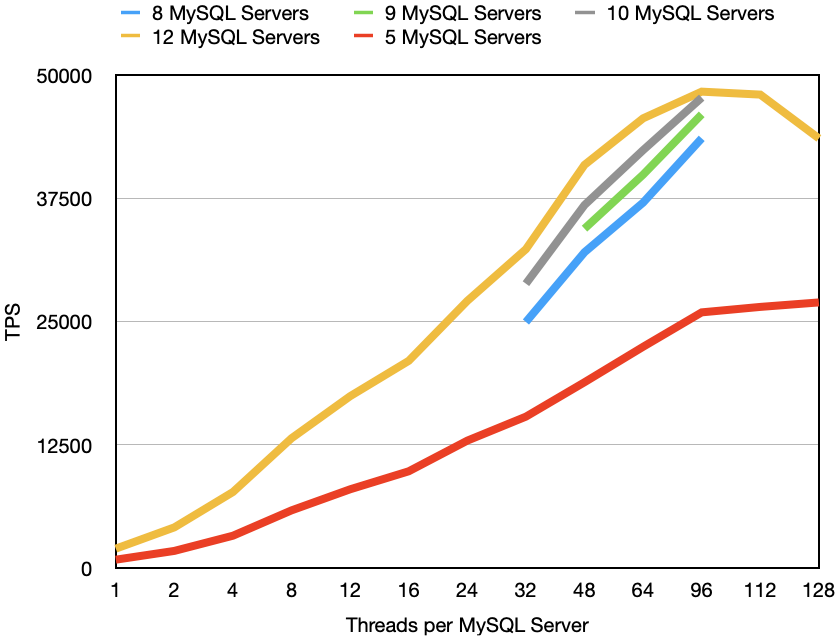
The graph below shows the throughput results from the larger data nodes using 8-12 MySQL Server VMs. Now in order to make sense of these numbers we will explain a bit more about Sysbench and how you can tweak Sysbench to serve your purposes for testing RonDB.


Description of Sysbench OLTP RW

The Sysbench OLTP RW benchmark consists of 20 SQL queries. There is a transaction, this means that the transaction starts with a BEGIN statement and it ends with a COMMIT statement. After the BEGIN statement follows 10 SELECT statements that selects one row using the primary key of the table. Next follows 4 SELECT queries that select 100 rows within a range and either uses SELECT DISTINCT, SELECT … ORDER BY, SELECT or SELECT sum(..). Finally there is one INSERT, one DELETE and 2 UPDATE queries.


In Pseudo code thus:

BEGIN

Repeat 10 times: SELECT col(s) from TAB where PK=pk

SELECT col(s) from TAB where key >= start AND key < (start + 100)

SELECT DISTINCT col(s) from TAB where key >= start AND key < (start + 100)

SELECT col(s) from TAB where key >= start AND key < (start + 100) ORDER BY key

SELECT SUM(col) from TAB where key >= start AND key < (start + 100)

INSERT INTO TAB values (....)

UPDATE TAB SET col=val WHERE PK=pk

UPDATE TAB SET col=val WHERE key=key

DELETE FROM TAB WHERE PK=pk

COMMIT 


This is the standard OLTP RW benchmark.

Benchmark Execution

Now I will describe some changes that the Sysbench installation in RonDB can handle. To understand this we will start by showing the default configuration file for Sysbench.


#

# Software definition

#

MYSQL_BIN_INSTALL_DIR="/srv/hops/mysql"

BENCHMARK_TO_RUN="sysbench"

#

# Storage definition (empty here)

#

#

# MySQL Server definition

#

SERVER_HOST="172.31.23.248;172.31.31.222"

MYSQL_PASSWORD='3*=13*8@20.*0@7$?=45'

#

# NDB node definitions (empty here)

#

#

# Benchmark definition

#

SYSBENCH_TEST="oltp_rw"

SYSBENCH_INSTANCES="2"

THREAD_COUNTS_TO_RUN="1;2;4;8;12;16;24;32;48;64;96;112;128"

MAX_TIME="30"


In this configuration file we provide the pointer to the RonDB binaries, we provide the type of benchmark we want to execute, we provide the password to the MySQL Servers, we provide the number of threads to execute in each step of the benchmark. There is also a list of IP addresses to the MySQL Servers in the cluster and finally we provide the number of instances of Sysbench we want to execute.


This configuration file is created automatically by the managed version of RonDB. This configuration file is available in the API nodes you created when you created the cluster. They are also available in the MySQL Server VMs if you want to test running with a single MySQL Server colocated with the application.


The default setup will run the standard Sysbench OLTP RW benchmark with one sysbench instance per MySQL Server. To execute this benchmark the following steps are done:


Step 1: Log in to the API node VM where you want to run the benchmark from. The username is ubuntu (in AWS). Thus log in using e.g. ssh ubuntu@IP_address. The IP address is the external IP address that you will find in AWS where your VM instances are listed.


Step 2: After successfully being logged in you need to log into the mysql user using the command:

sudo su - mysql


Step 3: Move to the right directory

cd benchmarks


Step 4: Execute the benchmark

bench_run.sh --default-directory /home/mysql/benchmarks/sysbench_multi

Benchmark Results

As you will discover there is also a sysbench_single, dbt2_single, dbt2_multi directory. These are setup for different benchmarks that we will describe in future papers. sysbench_single is the same as sysbench_multi but with only a single MySQL Server. This will exist also on MySQL Server VMs if you want to benchmark from those. Executing a benchmark from the sysbench machine increases latency since it represents a 3-tiered setup whereas executing sysbench in the MySQL Server represents a 2-tiered setup and thus the latency is lower.


If you want to study the benchmark in real-time repeat Step 1, 2 and 3 above and then perform the following commands:

cd sysbench_multi/sysbench_results

tail -f oltp_rw_0_0.res


This will display the output from the first sysbench instance that will provide latency numbers and throughput of one of the sysbench instances.


When the benchmark has completed the total throughput is found in the file:

/home/mysql/benchmarks/sysbench_multi/final_results.txt

Modifying Sysbench benchmark

The configuration for sysbench_multi is found in:

/home/mysql/benchmarks/sysbench_multi/autobench.conf


Thus if you want to modify the benchmark you can edit this file.


So how can we modify this benchmark. First you can decide on how many SELECT statements to retrieve using the primary key that should be issued. The default is 10. To change this add the following line in autobench.conf:

SB_POINT_SELECTS=”5”

This will change such that instead 5 primary key SELECTs will be issued for each transaction.


Next you can decide that you want those primary key SELECTs to retrieve a batch of primary keys. In this case the SELECT will use IN (key1, key2,,, keyN) in the WHERE clause. To use this set the number of keys to retrieve per statement in SB_USE_IN_STATEMENT. Thus to set this to 100 add the following line to autobench.conf.


SB_USE_IN_STATEMENT=”100”


This means that if SB_POINT_SELECTS is set to 5 and SB_USE_IN_STATEMENT is set to 100 there will be 500 key lookups performed per Sysbench OLTP transaction.


Next it is possible to set the number of range scan SELECTs to perform per transaction. So to e.g. disable all range scans we can add the following lines to autobench.conf.


SB_SIMPLE_RANGES=”0”

SB_ORDER_RANGES=”0”

SB_DISTINCT_RANGES=”0”

SB_SUM_RANGES=”0”


Now it is also possible to modify the range scans. I mentioned that the range scans retrieves 100 rows. The number 100 is changeable through the configuration parameter SB_RANGE_SIZE.


The default behaviour is to retrieve all 100 rows and send them back to the application. Thus no filtering. We also have an option to perform filtering in those range scans. In this case only 1 row will be returned, but we will still scan the number of rows specified in SB_RANGE_SIZE. This feature of Sysbench is activated through adding the following line to autobench.conf:


SB_USE_FILTER=”yes”


Finally it is possible to remove the use of INSERT, DELETE and UPDATEs. This is done by changing the configuration parameter SYSBENCH_TEST from oltp_rw to oltp_ro.


There are many more ways to change the configuration of how to run Sysbench, but these settings are enough for this paper. For more details see the documentation of dbt2-0.37.50, also see the Sysbench tree

Benchmark Configurations

In my benchmarking reported in this paper I used 2 different configurations. Later we will report more variants of Sysbench testing as well as other benchmark variants.


The first is the standard Sysbench OLTP RW configuration. The second is the standard benchmark but adding SB_USE_FILTER=”yes”. This was added since the standard benchmark becomes limited by the network bandwidth using r5.8xlarge instances for the data node. This instance type is limited to 10G Ethernet and it needs almost 20 Gb/s in networking capacity with the performance that RonDB delivers. This bandwidth is achievable using the r5n instances.


Each test of Sysbench creates the tables and fills them with data. To have a reasonable execution time of the benchmark each table will be filled with 1M rows. Each sysbench instance will use its own table. It is possible to set the number of rows per table, it is also possible to use multiple tables per sysbench instance. Here we have used the default settings.


The test runs are executed for a fairly short time to be able to test a large variety of test cases. This means that it is expected that results are a bit better than expected. To see how results are affected by running for a long time we also ran a few select tests where we ran a single benchmark for more than 1 hour. The results are in this case around 10% lower than the numbers of shorter runs. This is mainly due to variance of the throughput that is introduced by the execution of checkpoints in RonDB. Checkpoints consume around 5-10% of the CPU capacity in the RonDB data nodes.

Benchmark setup

In all tests set up here we have started the RonDB cluster using the Hopsworks infrastructure. In all tests we have used c5.4xlarge as the VM instance type for MySQL Servers. This VM has 16 VCPUs and 32 GB of memory. This means a VM with more or less 8 Intel Xeon CPU cores. In all tests there are 2 RonDB data nodes, we have tested with 2 types of VM instances here, the first is the r5.4xlarge which has 16 VCPUs with 128 GB of memory. The second is the r5n.8xlarge which has 32 VCPUs and 256 GB of memory. In the Standard Sysbench OLTP RW test the network became a bottleneck when using r5.8xlarge. These VMs can use up to 10 Gb/sec, but in reality we could see that some instances could not go beyond 7 Gb/sec, when switching to r5n.8xlarge instead this jumped up to 13Gb/sec immediately, so clearly this bottleneck was due to the AWS infrastructure.


To ensure that the network bottleneck was removed we switched to using r5n.8xlarge instances instead for those benchmarks. These instances are the same as r5.8xlarge except that they can use up to 25 Gb/sec in network bandwidth instead of 10Gb/sec.

Standard Sysbench OLTP RW

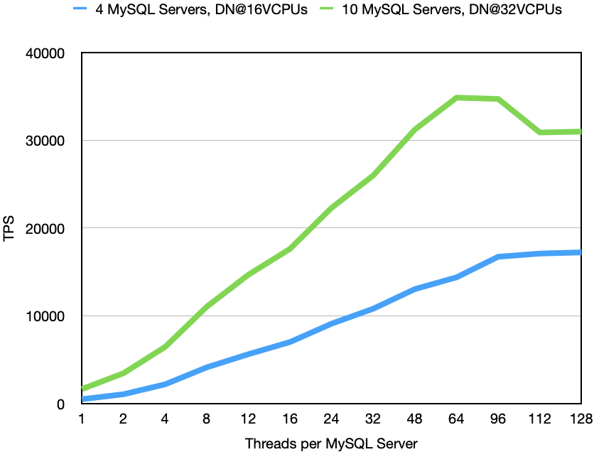
The first test we present here is the standard OLTP RW benchmark. When we run this benchmark most of the CPU consumption happens in the MySQL Servers. Each MySQL Server is capable of processing about 4000 TPS for this benchmark. The MySQL Server can process a bit more if the responsiveness of the data node is better, this is likely to be caused by that the CPU caches are hotter in that case when the response comes back to the MySQL Server. Two 16 VCPU data nodes can in this case handle the load from 4 MySQL Servers, adding a 5th can increase the performance slightly, but not much. We compared this to 2 data nodes using 32 VCPUs and in principle the load these data nodes could handle was doubled.


The response time was very similar in both cases, at extreme loads the larger data nodes had more latency increases, most likely due to the fact that we got much closer to the limits of what the network could handle.


The top number here was 34870 at 64 threads from 10 MySQL Servers. In this case 95% of the transactions had a latency that was less than 19.7 ms, this means that the time for each SQL query was below 1 millisecond. This meant that almost 700k SQL queries per second were executed. These queries reported back to the application 14.5M rows per second for the larger data nodes, most of them coming from the 4 range scan queries in the benchmark. Each of those rows are a bit larger than 100 bytes, thus around 2 GByte per second of application data is transferred to the application (about 25% of this is aggregated in the MySQL when using the SUM range scan).

Sysbench OLTP RW with filtering of scans

Given that Sysbench OLTP RW is to a great extent a networking test we also wanted to perform a test that performed a bit more processing, but reporting back a smaller amount of rows. We achieved this by setting SB_USE_FILTER=”yes” in the benchmark configuration file. This means that instead of each range scan SELECT reporting back 100 rows, it will read 100 rows and filter out 99 of them and report only 1 of the 100 rows. This will decrease the amount of rows to process down to about 1M rows per second. Thus this test is a better evaluator of the CPU efficiency of RonDB whereas the standard Sysbench OLTP RW is a good evaluator of RonDBs ability to ship tons of rows between the application and the database engine.


At first we wanted to see the effect the number of MySQL servers had on the throughput in this benchmark. We see the results of this in the image above. We see that there is an increase in throughput going from 8 to 12 MySQL Servers. However the additional effect of each added MySQL Server is diminishing. There is very little to gain going beyond 10 MySQL Servers. The optimal use of computing resources is most likely achieved around 8-9 MySQL Servers.

Adding additional MySQL servers also has an impact on the variability of the latency. So probably the overall best fit here is to use about 2x more CPU resources on the MySQL Servers compared to the CPU resources in the RonDB data nodes. This rule is based on this benchmark and isn’t necessarily true for another use case.


The results with the smaller data nodes, r5.4xlarge is the red line that used 5 MySQL Servers in the test.


The rule definitely changes when using the key-value store APIs that RonDB provides. These are at least 100% more efficient compared to using SQL.


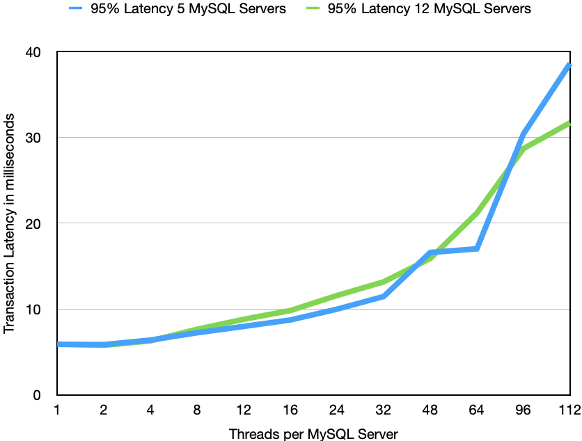
A key-value store needs to be a LATS database (low Latency, high Availability, high Throughput, Scalable storage). In this paper we have focused on showing Throughput and Latency. Above is the graph showing how latency is affected by the number of threads in the MySQL Server.


Many applications have strict requirements on the maximum latency of transactions. So for example if the application requires response time to be smaller than 20 ms than we can see in the graph that we can use around 60 threads towards each MySQL Server. At this number of threads r5.4xlarge delivers 22500 TPS (450k QPS) and r5n.8xlarge delivers twice that number, 45000 TPS (900k QPS).


The base latency in an unloaded cluster is a bit below 6 milliseconds. This number is a bit variable based on where exactly the VMs are located that gets started for you. Most of this latency is spent in latency on the networks.  Each network jump in AWS has been reported to be around 40-50 microseconds and one transaction performs around 100 of those network jumps in sequence. Thus almost two-thirds of the base latency comes from the latency in getting messages across. At higher loads the queueing waiting the message to be executed becomes dominating. Benchmarks where everything executes on a single computer has base latency around 2 millisecond per Sysbench transaction which confirms the above calculations.