Showing posts with label benchmarks. Show all posts

Monday, May 27, 2024

875X improvement from RonDB 21.04.17 to 22.10.4

At Hopsworks we are working on ensuring that the online feature store will be able to perform complex join operations in real-time. This means that queries that could use data from multiple tables can be easily integrated into machine learning applications.

Today most feature stores use key-value stores like Redis and DynamoDB. These systems have no capability to issue complex join queries, if this is required the feature store will have to write complex code to handle this and this is likely to involve multiple roundtrips and thus cause unwanted latency.

Hopsworks feature store uses RonDB as its online feature store. RonDB can handle any SQL operations that MySQL can handle. Actually RonDB has even support for parallelising the join queries and pushing the filtering and joining down to the RonDB data nodes where data resides.

This means that users of the Hopsworks feature store can integrate more features from multiple feature groups in online inferencing requests. This means that things credit fraud detection can be made much more intelligent by taking more features into account in the inferencing requests.

This means that performance of real-time join queries becomes more important in RonDB. To evaluate how RonDB develops in this are I ran a set of tests using TPC-H queries from DBT3 against RonDB 21.04.17 and RonDB 22.10.4 (not released yet). I also ran tests against MySQL 8.0.35 (RonDB 22.10.4 is based on MySQL 8.0.35 with loads of added RonDB features).

The results were interesting, the improvement in Q20 was the highest I have seen in my career. The performance improved from 70 seconds to 80 milliseconds, thus an 875x speedup or 87500% improvement. Q2 had a 360x improvement. So RonDB 22.10.4 is much better equipped for more complex queries compared to RonDB 21.04. MySQL 8.0.35 had similar performance to RonDB 22.10.4 with an average of around 20% slower, this is mostly due to performance improvements in RonDB, not algorithmic changes.

When using complex queries the query optimiser tries to find an optimal plan, sometimes however better plans are available and one can add hints in the SQL query to ensure a better plan is used.

The RonDB team isn't satisfied with this however, we have realised that evaluating aggregation is also very important when the online feature store stores a time window of certain features. This means that RonDB can compute aggregate dynamically and thus provide more accurate predictions.

Early tests of some simple single table queries showed an improvement of 4-5x and we expect we will be able to get to 10-20x improvements in quite a few queries of this sort.

Thursday, October 26, 2023

Results on comparing new Intel/AMD VMs with older VM types using RonDB

 In Hopsworks cloud offering for GCP one can select a fairly large variety of VM types. I am currently working on extending this list to also include the latest generation of VM types. This blog will focus on the impact of those new VM types for benchmarks using RonDB.

The newer VM types is the c3d-serie that uses AMD EPYC CPUs of the 4th generation and the c3-series which contains VMs using the Intel Saphire Rapid CPUs. Also AWS has introduced similar new VM types, but this blog discuss tests performed on VMs in GCP.

The older VM types we compared with for the MySQL Servers was the n2-standard-16 VM type. This VM uses an Intel Cascade Lake Xeon processor. This represents the second generation Intel Xeon chips whereas Intel Saphire Rapid represents the 4th generation Intel Xeon.

The RonDB data nodes used the e2-highmem-16 as the baseline for comparison. This VM types uses either an Intel Xeon of the second generation or an AMD EPYC of the second generation.

The benchmark used was Sysbench OLTP RW based on version 0.4.12.19 which is included in the RonDB tarball and is setup in the API nodes automatically by our cloud offering. This makes it extremely easy to replicate the benchmarks. We use Consul as a load balancer, so the benchmark process is setup to a single host onlinefs.mysql.service.consul. In reality this address maps to the number of MySQL Servers in the RonDB cluster. We used 3 MySQL Servers in the tests. The setup used 2 RonDB data nodes in one node group.

Thus in the Hopsworks cloud we get a load balanced RonDB Data Service as part of the infrastructure of the Hopsworks Feature Store.

We first executed the benchmark using the old VM types to get a baseline. The next step was to upgrade the RonDB MySQL Servers to use c3d-highmem-16. Thus the same amount of memory and number of CPUs as in n2-standard-16 but upgraded from Intel 2nd generation to AMD 4th generation.

This impacted the throughput mainly. The baseline experiment executed 9000 TPS and was limited by the CPUs in the MySQL Servers (they used 1550% of the 1600% available). The c3d-highmem-16 delivered 11400 TPS but only using 1000% of the available 1600%. Thus the throughput per CPU increased by around 100%. In this execution the bottleneck of the benchmark was the RonDB data nodes.

The benchmark API node was consistently a n2-standard-48 VM. This meant that most communication went from API VM of old type, to MySQL Server of new type, to RonDB data node VM of old type. Thus in all communication an old VM type was involved. The network latency was the same in this experiment as in the baseline experiment.

The change from one VM type was using the Reconfiguration support RonDB have in its Cloud offering. This change is an online operation where the cluster remains operational and the new MySQL Servers are included in the Consul setup as soon as they have started up. Only when nodes are stopped could temporary errors happen that can be handled with a simple retry logic.

Next we changed also the VM type of the RonDB data nodes to be c3d-highmem-16 using the same online reconfiguration as for the MySQL Servers.

What we quickly noted in this setup was that the latency per transaction was cut in half. Thus performance using a single thread decreased to less than half. Thus it is clear that communication between 2 VMs of the new type have more than 100% improvements on network latency. The throughput now increased to 17800 TPS and the bottleneck was now in the MySQL Servers. Thus throughput improvement is almost 98% and network latency improved by more than 100%.

When reading the announcement of the C3 machine series and the description of the C3D machine series, it is clear that the new IPU (Infrastructure Processing Unit) that takes care of offloading networking is a major reason for this improved network latency.

Analysing the Sysbench transaction in this setup there will be around 100 network messages, most of them in serial order. Still the latency of a transaction execution is no more than 6 milliseconds to execute the 20 SQL queries involved in the OLTP RW transaction. Thus a medium of 60 microsecond per message and this includes the time to also execute the RonDB Data node code and the RonDB MySQL Server code.

Next step was to again change MySQL Server VMs. This time we changed to c3-highmem-22. Unfortunately the VM type c3-highmem-16 didn't exist. So the comparison isn't perfect, but at least it gives a good estimate of the improvements in Intel's 4th generation CPUs.

The network latency was the same for Intel and AMD 4th generation VM types. The throughput increased by around 40% up to around 24000 TPS. Since the number of CPUs increased by around 40% as well, it seems that c3-serie and c3d-serie is very similar in handling throughput when used in RonDB MySQL Servers.

To test the throughput of those new VMs we ran the test using c3-highmem-8 and c3d-highmem-8 VM types as RonDB Data node VMs. The performance of those two VM types was almost indistinguishable, to the point where I started wondering if they were the same CPUs. Throughput was half the throughput of the 16 VCPU VMs.

The main conclusion of these tests is that upgrading from 2nd generation x86 CPUs to 4th generation x86 CPUs in the GCP cloud provides a 100% improvement in throughput and a similar improvement of the network latency.

The price of those VMs is higher, but substantially less than 100%. So it makes a lot of sense to start using those new VM types for new applications.

The tests were performed using the RonDB version 21.04.15. We are about to release a new LTS version of RonDB, version 22.10.1. There will be a more thorough benchmark report when this is released.

Thursday, March 23, 2023

Laptop vs Desktop for RonDB development

 Most developers today use laptops for all development work. For the last 15 years I have considered desktops and laptops to be very similar in performance and use cases. This is no longer the case as I will discuss in this blog.

Personally I use a mix of laptops and desktops. For me the most important thing as a developer is the screen resolution and the speed of compilation. But I have now found that desktops can be very useful for the test phase of a development project, in particular the later testing phases.

Many years ago I read that one can increase productivity by 30% by using a screen with higher resolution thus fitting more things at the same time on the screen. Personally I have so far found 27" screens to be the best size, larger size means neck pain and smaller means that productivity suffers. The screen resolution should be as high as your budget allows.

My experience is that modern laptops can be quite efficient in compilation. There is very little difference in compilation time towards desktops.

However recently I tested running our new RonDB Docker clusters on laptops and desktops. What I have seen is that the performance of these tests can differ up to 4x.

I think the reason for this large difference is that desktops can sustain high performance for a long time. Some modern desktops can handle CPUs that use more than 200W whereas most laptops will be limited to about 45W. For a compilation that only runs for about 5 minutes and have some serialisation the difference becomes very small. The most important part for compilation is how fast the CPU is on single-threaded performance and that it can scale the compilation to a decent number of CPUs.

However running a development environment for RonDB means running a cluster on a single machine where there are two data node processes, two MySQL server processes and a management process and of course any number of application processes. A laptop can handle this nicely and the performance for a single-threaded application is the same for laptop and desktop. However when scaling the test to many threads the laptop hits a wall whereas the desktop simply continues to scale.

The reason is twofold, the desktop CPUs can have more CPU cores. Most high-end laptops today have around 8-10 CPU cores. The high-end desktops today however goes to around 16-24 CPU cores. In addition the desktop can usually handle more than 4x as much power. The power difference and the core difference delivers a 4x higher throughput in heavy testing.

Thus my conclusion is that laptops are good enough for the development phase together with an external screen. However when you enter the testing phase when you need to run heavy functional tests and load tests on your software a desktop or a workstation will be very useful.

In my tests on a high-end desktop I ran a Sysbench OLTP RW benchmark using the RonDB Docker environment, I managed to run up to 15.000 TPS. This means running 300.000 SQL queries per second towards the MySQL servers and the data nodes. The laptop could handle roughly 25% of this throughput.

Obviously the desktop could be a virtual desktop in the modern development environment. But a physical machine is still a lot more fun.

RonDB is part of the Hopsworks Feature Store platform.


Wednesday, May 05, 2021

Sysbench evaluation of RonDB


Introduction

Sysbench is a tool to benchmark to test open source databases. We have integrated Sysbench into the RonDB installation. This makes it extremely easy to run benchmarks with RonDB. This paper will describe the use of these benchmarks in RonDB. These benchmarks were executed with 1 cluster connection per MySQL Server. This limited the scalability per MySQL Server to about 12 VCPUs. Since we executed those benchmarks we have increased the number of cluster connections per MySQL Server to 4 providing scalability to at least 32 VCPUs per MySQL Server.


As preparation to run those benchmarks we have created a RonDB cluster using the Hopsworks framework that is currently used to create RonDB clusters. In these tests all MySQL Servers are using the c5.4xlarge VM instances in AWS (16 VCPUs with 32 GB memory). We have a RonDB management server using the t3a.medium VM instance type. We have tested using two different RonDB clusters, both have 2 data nodes. The first test is using the r5.4xlarge instance type (16 VCPUs and 128 GB memory) and the second test uses the r5n.8xlarge (32 VCPUs and 256 GB memory). It was necessary to use r5n class since we needed more than 10Gbit/second network bandwidth for the OLTP RW test with 32 VCPUs on data nodes.


In the RonDB documentation you can find more details how to set up your own RonDB cluster in either our managed version (currently supporting AWS) or using our open source shell scripts to set up a cluster (currently supporting GCP and Azure). RonDB is a new distribution of MySQL NDB Cluster. All experiments in this blog was performed using RonDB 21.04.0.


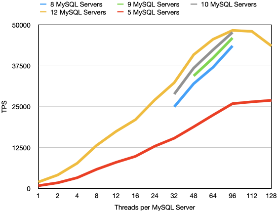
The graph below shows the throughput results from the larger data nodes using 8-12 MySQL Server VMs. Now in order to make sense of these numbers we will explain a bit more about Sysbench and how you can tweak Sysbench to serve your purposes for testing RonDB.


Description of Sysbench OLTP RW

The Sysbench OLTP RW benchmark consists of 20 SQL queries. There is a transaction, this means that the transaction starts with a BEGIN statement and it ends with a COMMIT statement. After the BEGIN statement follows 10 SELECT statements that selects one row using the primary key of the table. Next follows 4 SELECT queries that select 100 rows within a range and either uses SELECT DISTINCT, SELECT … ORDER BY, SELECT or SELECT sum(..). Finally there is one INSERT, one DELETE and 2 UPDATE queries.


In Pseudo code thus:

BEGIN

Repeat 10 times: SELECT col(s) from TAB where PK=pk

SELECT col(s) from TAB where key >= start AND key < (start + 100)

SELECT DISTINCT col(s) from TAB where key >= start AND key < (start + 100)

SELECT col(s) from TAB where key >= start AND key < (start + 100) ORDER BY key

SELECT SUM(col) from TAB where key >= start AND key < (start + 100)

INSERT INTO TAB values (....)

UPDATE TAB SET col=val WHERE PK=pk

UPDATE TAB SET col=val WHERE key=key

DELETE FROM TAB WHERE PK=pk

COMMIT 


This is the standard OLTP RW benchmark.

Benchmark Execution

Now I will describe some changes that the Sysbench installation in RonDB can handle. To understand this we will start by showing the default configuration file for Sysbench.


#

# Software definition

#

MYSQL_BIN_INSTALL_DIR="/srv/hops/mysql"

BENCHMARK_TO_RUN="sysbench"

#

# Storage definition (empty here)

#

#

# MySQL Server definition

#

SERVER_HOST="172.31.23.248;172.31.31.222"

MYSQL_PASSWORD='3*=13*8@20.*0@7$?=45'

#

# NDB node definitions (empty here)

#

#

# Benchmark definition

#

SYSBENCH_TEST="oltp_rw"

SYSBENCH_INSTANCES="2"

THREAD_COUNTS_TO_RUN="1;2;4;8;12;16;24;32;48;64;96;112;128"

MAX_TIME="30"


In this configuration file we provide the pointer to the RonDB binaries, we provide the type of benchmark we want to execute, we provide the password to the MySQL Servers, we provide the number of threads to execute in each step of the benchmark. There is also a list of IP addresses to the MySQL Servers in the cluster and finally we provide the number of instances of Sysbench we want to execute.


This configuration file is created automatically by the managed version of RonDB. This configuration file is available in the API nodes you created when you created the cluster. They are also available in the MySQL Server VMs if you want to test running with a single MySQL Server colocated with the application.


The default setup will run the standard Sysbench OLTP RW benchmark with one sysbench instance per MySQL Server. To execute this benchmark the following steps are done:


Step 1: Log in to the API node VM where you want to run the benchmark from. The username is ubuntu (in AWS). Thus log in using e.g. ssh ubuntu@IP_address. The IP address is the external IP address that you will find in AWS where your VM instances are listed.


Step 2: After successfully being logged in you need to log into the mysql user using the command:

sudo su - mysql


Step 3: Move to the right directory

cd benchmarks


Step 4: Execute the benchmark

bench_run.sh --default-directory /home/mysql/benchmarks/sysbench_multi

Benchmark Results

As you will discover there is also a sysbench_single, dbt2_single, dbt2_multi directory. These are setup for different benchmarks that we will describe in future papers. sysbench_single is the same as sysbench_multi but with only a single MySQL Server. This will exist also on MySQL Server VMs if you want to benchmark from those. Executing a benchmark from the sysbench machine increases latency since it represents a 3-tiered setup whereas executing sysbench in the MySQL Server represents a 2-tiered setup and thus the latency is lower.


If you want to study the benchmark in real-time repeat Step 1, 2 and 3 above and then perform the following commands:

cd sysbench_multi/sysbench_results

tail -f oltp_rw_0_0.res


This will display the output from the first sysbench instance that will provide latency numbers and throughput of one of the sysbench instances.


When the benchmark has completed the total throughput is found in the file:

/home/mysql/benchmarks/sysbench_multi/final_results.txt

Modifying Sysbench benchmark

The configuration for sysbench_multi is found in:

/home/mysql/benchmarks/sysbench_multi/autobench.conf


Thus if you want to modify the benchmark you can edit this file.


So how can we modify this benchmark. First you can decide on how many SELECT statements to retrieve using the primary key that should be issued. The default is 10. To change this add the following line in autobench.conf:

SB_POINT_SELECTS=”5”

This will change such that instead 5 primary key SELECTs will be issued for each transaction.


Next you can decide that you want those primary key SELECTs to retrieve a batch of primary keys. In this case the SELECT will use IN (key1, key2,,, keyN) in the WHERE clause. To use this set the number of keys to retrieve per statement in SB_USE_IN_STATEMENT. Thus to set this to 100 add the following line to autobench.conf.


SB_USE_IN_STATEMENT=”100”


This means that if SB_POINT_SELECTS is set to 5 and SB_USE_IN_STATEMENT is set to 100 there will be 500 key lookups performed per Sysbench OLTP transaction.


Next it is possible to set the number of range scan SELECTs to perform per transaction. So to e.g. disable all range scans we can add the following lines to autobench.conf.


SB_SIMPLE_RANGES=”0”

SB_ORDER_RANGES=”0”

SB_DISTINCT_RANGES=”0”

SB_SUM_RANGES=”0”


Now it is also possible to modify the range scans. I mentioned that the range scans retrieves 100 rows. The number 100 is changeable through the configuration parameter SB_RANGE_SIZE.


The default behaviour is to retrieve all 100 rows and send them back to the application. Thus no filtering. We also have an option to perform filtering in those range scans. In this case only 1 row will be returned, but we will still scan the number of rows specified in SB_RANGE_SIZE. This feature of Sysbench is activated through adding the following line to autobench.conf:


SB_USE_FILTER=”yes”


Finally it is possible to remove the use of INSERT, DELETE and UPDATEs. This is done by changing the configuration parameter SYSBENCH_TEST from oltp_rw to oltp_ro.


There are many more ways to change the configuration of how to run Sysbench, but these settings are enough for this paper. For more details see the documentation of dbt2-0.37.50, also see the Sysbench tree

Benchmark Configurations

In my benchmarking reported in this paper I used 2 different configurations. Later we will report more variants of Sysbench testing as well as other benchmark variants.


The first is the standard Sysbench OLTP RW configuration. The second is the standard benchmark but adding SB_USE_FILTER=”yes”. This was added since the standard benchmark becomes limited by the network bandwidth using r5.8xlarge instances for the data node. This instance type is limited to 10G Ethernet and it needs almost 20 Gb/s in networking capacity with the performance that RonDB delivers. This bandwidth is achievable using the r5n instances.


Each test of Sysbench creates the tables and fills them with data. To have a reasonable execution time of the benchmark each table will be filled with 1M rows. Each sysbench instance will use its own table. It is possible to set the number of rows per table, it is also possible to use multiple tables per sysbench instance. Here we have used the default settings.


The test runs are executed for a fairly short time to be able to test a large variety of test cases. This means that it is expected that results are a bit better than expected. To see how results are affected by running for a long time we also ran a few select tests where we ran a single benchmark for more than 1 hour. The results are in this case around 10% lower than the numbers of shorter runs. This is mainly due to variance of the throughput that is introduced by the execution of checkpoints in RonDB. Checkpoints consume around 5-10% of the CPU capacity in the RonDB data nodes.

Benchmark setup

In all tests set up here we have started the RonDB cluster using the Hopsworks infrastructure. In all tests we have used c5.4xlarge as the VM instance type for MySQL Servers. This VM has 16 VCPUs and 32 GB of memory. This means a VM with more or less 8 Intel Xeon CPU cores. In all tests there are 2 RonDB data nodes, we have tested with 2 types of VM instances here, the first is the r5.4xlarge which has 16 VCPUs with 128 GB of memory. The second is the r5n.8xlarge which has 32 VCPUs and 256 GB of memory. In the Standard Sysbench OLTP RW test the network became a bottleneck when using r5.8xlarge. These VMs can use up to 10 Gb/sec, but in reality we could see that some instances could not go beyond 7 Gb/sec, when switching to r5n.8xlarge instead this jumped up to 13Gb/sec immediately, so clearly this bottleneck was due to the AWS infrastructure.


To ensure that the network bottleneck was removed we switched to using r5n.8xlarge instances instead for those benchmarks. These instances are the same as r5.8xlarge except that they can use up to 25 Gb/sec in network bandwidth instead of 10Gb/sec.

Standard Sysbench OLTP RW

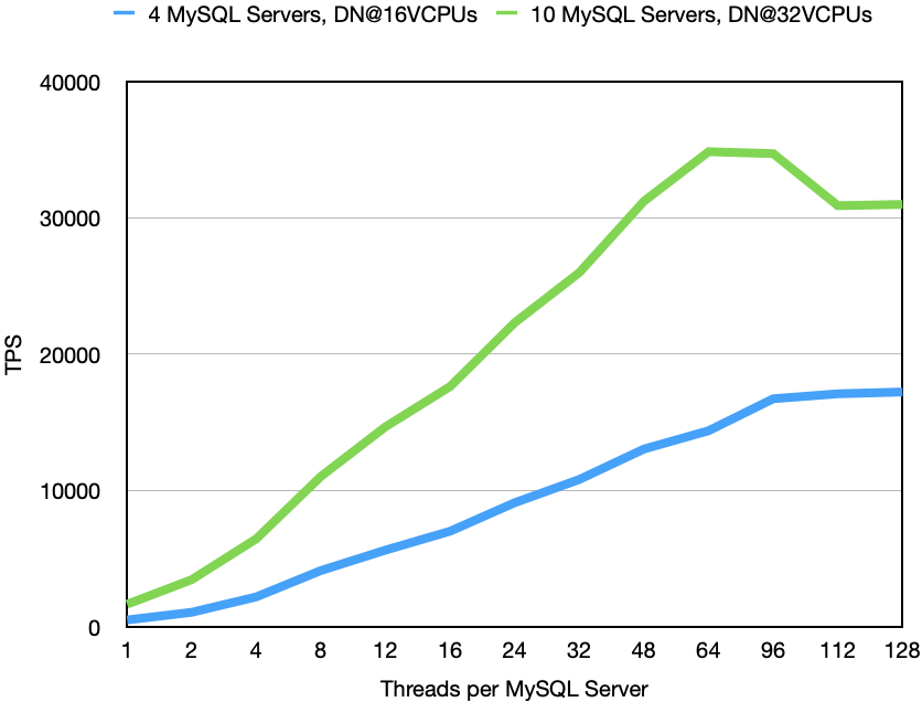
The first test we present here is the standard OLTP RW benchmark. When we run this benchmark most of the CPU consumption happens in the MySQL Servers. Each MySQL Server is capable of processing about 4000 TPS for this benchmark. The MySQL Server can process a bit more if the responsiveness of the data node is better, this is likely to be caused by that the CPU caches are hotter in that case when the response comes back to the MySQL Server. Two 16 VCPU data nodes can in this case handle the load from 4 MySQL Servers, adding a 5th can increase the performance slightly, but not much. We compared this to 2 data nodes using 32 VCPUs and in principle the load these data nodes could handle was doubled.


The response time was very similar in both cases, at extreme loads the larger data nodes had more latency increases, most likely due to the fact that we got much closer to the limits of what the network could handle.


The top number here was 34870 at 64 threads from 10 MySQL Servers. In this case 95% of the transactions had a latency that was less than 19.7 ms, this means that the time for each SQL query was below 1 millisecond. This meant that almost 700k SQL queries per second were executed. These queries reported back to the application 14.5M rows per second for the larger data nodes, most of them coming from the 4 range scan queries in the benchmark. Each of those rows are a bit larger than 100 bytes, thus around 2 GByte per second of application data is transferred to the application (about 25% of this is aggregated in the MySQL when using the SUM range scan).

Sysbench OLTP RW with filtering of scans

Given that Sysbench OLTP RW is to a great extent a networking test we also wanted to perform a test that performed a bit more processing, but reporting back a smaller amount of rows. We achieved this by setting SB_USE_FILTER=”yes” in the benchmark configuration file. This means that instead of each range scan SELECT reporting back 100 rows, it will read 100 rows and filter out 99 of them and report only 1 of the 100 rows. This will decrease the amount of rows to process down to about 1M rows per second. Thus this test is a better evaluator of the CPU efficiency of RonDB whereas the standard Sysbench OLTP RW is a good evaluator of RonDBs ability to ship tons of rows between the application and the database engine.


At first we wanted to see the effect the number of MySQL servers had on the throughput in this benchmark. We see the results of this in the image above. We see that there is an increase in throughput going from 8 to 12 MySQL Servers. However the additional effect of each added MySQL Server is diminishing. There is very little to gain going beyond 10 MySQL Servers. The optimal use of computing resources is most likely achieved around 8-9 MySQL Servers.

Adding additional MySQL servers also has an impact on the variability of the latency. So probably the overall best fit here is to use about 2x more CPU resources on the MySQL Servers compared to the CPU resources in the RonDB data nodes. This rule is based on this benchmark and isn’t necessarily true for another use case.


The results with the smaller data nodes, r5.4xlarge is the red line that used 5 MySQL Servers in the test.


The rule definitely changes when using the key-value store APIs that RonDB provides. These are at least 100% more efficient compared to using SQL.


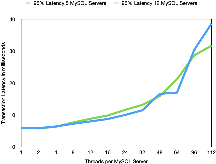
A key-value store needs to be a LATS database (low Latency, high Availability, high Throughput, Scalable storage). In this paper we have focused on showing Throughput and Latency. Above is the graph showing how latency is affected by the number of threads in the MySQL Server.


Many applications have strict requirements on the maximum latency of transactions. So for example if the application requires response time to be smaller than 20 ms than we can see in the graph that we can use around 60 threads towards each MySQL Server. At this number of threads r5.4xlarge delivers 22500 TPS (450k QPS) and r5n.8xlarge delivers twice that number, 45000 TPS (900k QPS).


The base latency in an unloaded cluster is a bit below 6 milliseconds. This number is a bit variable based on where exactly the VMs are located that gets started for you. Most of this latency is spent in latency on the networks.  Each network jump in AWS has been reported to be around 40-50 microseconds and one transaction performs around 100 of those network jumps in sequence. Thus almost two-thirds of the base latency comes from the latency in getting messages across. At higher loads the queueing waiting the message to be executed becomes dominating. Benchmarks where everything executes on a single computer has base latency around 2 millisecond per Sysbench transaction which confirms the above calculations.


Thursday, April 29, 2021

Comparing RonDB 21.04.0 on AWS, Azure and GCP using Sysbench


Release of RonDB 21.04.0

RonDB is based on MySQL NDB Cluster optimised for use in modern cloud settings. Today we launch RonDB 21.04.0. In RonDB 21.04.0 we have integrated benchmark scripts to execute various benchmarks towards RonDB.


There are three ways of using RonDB. The first is using the managed version provided by Logical Clocks. This is currently available in AWS and is currently being developed to also support Azure. This is still in limited access mode. To access it contact Logical Clocks at the rondb.com website.


The second way is to use a script provided by Logical Clocks that automates the creation of VMs and the installation of the software components required by RonDB. These scripts are available to create RonDB clusters on Azure and GCP (Google Cloud). This script can be downloaded from nexus.hops.works/rondb-cloud-installer.sh.


The third manner to use RonDB is to simply download the RonDB binary tarball and install it on any computers of your own liking.


All these methods start by visiting http://rondb.com. From here you will find the download scripts, the tarball to download and to send an email request access to the managed version of RonDB.


RonDB 21.04.0 can be used in any of the above settings, but we focus our development, testing and optimisations towards executing RonDB in an efficient manner in AWS, Azure and GCP. We will likely add Oracle Cloud eventually to the mix as well.


Benchmark Setup


What we have discovered in our benchmarking is that even with very similar HW there are some differences in how RonDB performs on the different clouds. So this report presents the results using very similar setups in AWS, Azure and GCP.
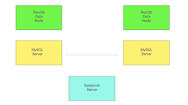
Above we have the benchmark setup used in all the experiments. There are always 2 RonDB data nodes and they are replicas of each other. Thus all write operations are written on both data nodes to ensure that we are always available even in the presence of node failures.


The MySQL Servers are pure clients since data is located on the RonDB data nodes. Thus we can easily scale the benchmark using any number of MySQL Servers. The benchmark application runs on a single VM that sends SQL queries to the MySQL Servers and receives results using a MySQL client written in C. It is sufficient to have a single Sysbench server for these experiments.


In this experiment we will scale RonDB data nodes by using different VM types. It is also possible to scale RonDB by adding more RonDB data nodes. Both of these changes can be performed without any downtime.


It is possible to execute the Sysbench server local to the MySQL Server and let multiple Sysbench servers execute in parallel. This would however be a 2-tiered cluster and we wanted to test a 3-tiered cluster setup since we think this is the most common setup used. Obviously a 2-tiered cluster setup will have lower latency, but it will also be more complex to maintain.


There is also a RonDB management server in the setup, however this is not involved in the benchmark execution and is either located in the Sysbench server or a separate dual CPU VM. 

Availability Zones

AWS, Azure and GCP all use a concept called Availability Zones. These are located in the same city, but can be distant from each other. The latency between Availability Zones can be more than 1 millisecond in latency for each jump. RonDB contains options to optimise for such a setup, but in this test we wanted to test a setup that is within an Availability Zone.


Thus all setups we ensured that all VMs participating in cluster setup were in the same zone. Even within a zone the variance on the latency can be substantial. We see this in that the benchmark numbers can vary even within the same cloud and the same availability zone on different runs. From other reports it is reported that network latency is around 40-60 microseconds between VMs in the same availability zone. Our experience is that it is normal that this latency varies at least 10-20 microseconds up or down. In Azure it is even possible that the variance is higher since they can implement some availability zones in multiple buildings. In this case Azure provides a concept called Proximity Placement Groups that can be used to ensure that VMs are located in the same building and not spread between buildings in the same availability zone.

RonDB VM Types


All cloud vendors have VMs that come from different generations of SW and HW. For a latency sensitive application like RonDB this had serious implications. All the VMs we tested used very similar Intel x86 CPUs. There is some difference in performance between older Intel x86 and newer CPUs. However this difference is usually on the order of 30-40%, so not so drastic.


However an area where innovation has happened at a much higher pace is networking. Cloud vendors have drastically improved the networking latency, bandwidth and efficiency from generation to generation.


What we found is that it is essential to use the latest VM generation for MySQL Servers and RonDB data nodes. The difference between the latest generation and the previous generation was up to 3x in latency and performance. We found that the latest generation of VMs from all cloud vendors have similar performance, but using older versions had a high impact on the benchmark results. All the benchmarking results in this report uses the latest generation of VMs from all vendors.


For AWS this means using their 5th generation VMs. AWS has three main categories of VMs, these c5, m5 and r5. c5 VMs are focused on lots of CPU and modest amounts of memory. m5 VMs twice as much memory with the same amount of CPU and r5 have 4x more memory than the c5 and the same amount of CPU. For RonDB this works perfectly fine. The RonDB data nodes store all the data and thus require as much memory as possible. Thus we use the r5 category here. MySQL Servers only act as clients in RonDB setup, thus require only a modest amount of memory, thus we use the c5 category here.


The latest generation in Azure is the v4 generation. Azure VMs have two categories, the D and E VMs. The E category has twice as much memory as the D category. The E category is similar to AWS r5 and the D category is similar to the AWS m5 category.


The latest generation in GCP is the n2 generation. They have n2-highcpu that matches AWS c5, n2-standard that matches AWS m5 and n2-highmem that matches AWS r5. GCP also has the ability to extend memory beyond 8 GB per CPU which is obviously interesting for RonDB.

Benchmark Notes on Cloud Vendors

Since we developed the RonDB managed version on AWS we have a bit more experience from benchmarking here. We quickly discovered that the standard Sysbench OLTP RW benchmark actually is not only a CPU benchmark. It is very much a networking benchmark as well. In some benchmarks using 32 VCPUs on the data nodes, we had to send around 20 Gb/sec from the data node VMs. Not all VM types could handle this. In AWS this meant that we had to use a category called r5n. This category uses servers that have 100G Ethernet instead of 25G Ethernet and thus a 32 VCPU VM was provided with bandwidth up to 25G. We didn’t investigate this thoroughly on Azure and GCP.


Some quirks we noted was that the supply of Azure v4 VM instances was somewhat limited. In some regions it was difficult to succeed in allocating a set of large v4 VM instances. In GCP we had issues with our quotas and got a denial to increase the quota size for n2 VMs, which was a bit surprising. This meant that we executed not as many configurations on Azure and GCP. Thus some comparisons are between Azure and AWS only.


Using the latest VM generation AWS, Azure and GCP all had reasonable performance. There were differences of course, but between 10-30% except in one benchmark. Our conclusion is that AWS, Azure and GCP have used different strategies in how to handle networking interrupts. AWS reports the lowest latency on networking in our tests and this is also seen in other benchmark reports. However GCP shows both in our benchmarks and other similar reports to have higher throughput but worse latency. Azure falls in between those.


Our conclusion is that it is likely caused by how network interrupts are handled. If the network interrupts are acted upon immediately one gets the best possible latency. But at high loads the performance goes down since interrupt handling costs lots of CPU. If network interrupts are instead handled using polling the latency is worse, but at high loads the cost of interrupts stays low even at extreme loads.


Thus best latency is achieved through handling interrupts directly and using polling one gets better performance the longer the delay in the network interrupt. Obviously the true answer is a lot more complex than this, but suffice it to say that the cloud vendors have selected different optimisation strategies that work well in different situations.

Benchmark Notes on RonDB


One more thing that affects latency of RonDB to a great extent is the wakeup latency of threads. Based on benchmarks I did while at Oracle I concluded that wakeup latency is about 2x higher on VMs compared to on bare metal. On VMs it can be as high as 25 microseconds, but is likely nowadays to be more like on the order of 10-15 microseconds.


RonDB implements adaptive CPU spinning. This ensures that latency is decreasing when the load increases. This means that we get a latency curve that starts a bit higher, then goes down until the queueing for CPU resources starts to impact latency and after that it follows a normal latency where latency increases as load increases.


Latency variations are very small up to about 50% of the maximum load on RonDB.


In our benchmarks we have measured the latency that 95% of the transactions were below. Thus we didn’t focus so much on single outliers. RonDB is implementing soft real-time, thus it isn’t intended for hard real-time applications where life depends on individual transactions completing in time.


The benchmarks do however report a maximum latency. Most of the time these maximum latencies were as expected. But one outlier we saw, this was on GCP where we saw transaction latency at a bit above 200 ms when executing benchmarks with up to 8 threads. These outliers disappeared when going towards higher thread counts. Thus it seems that GCP VMs have some sort of deep sleep that keeps them down for 200 ms. This latency was always in the range 200-210 milliseconds. Thus it seemed that there was a sleep of 200ms somewhere in the VM. In some experiments on Azure we saw even higher maximum latency with similar behaviour as on GCP. So it is likely that most cloud vendors (probably all) can go into deep sleeps that highly affect latency when operations start up again.

Benchmark Configuration

Ok, now on to numbers. We will show results from 4 different setups. All setups use 2 data nodes. The first setup uses 2 MySQL Servers and both RonDB data nodes and MySQL Servers use VMs with 16 VCPUs. This setup mainly tests latency and performance of MySQL Servers in an environment where data nodes are not overloaded. This test compares AWS, Azure and GCP.


The second setup increases the number of MySQL Servers to 4 in the same setup. This makes the data node the bottleneck in the benchmark. This benchmark also compares AWS, Azure and GCP.


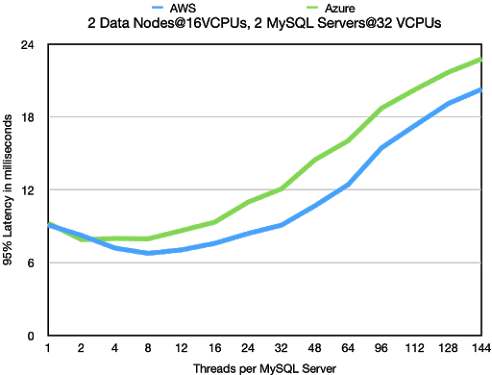
The third setup uses 16 VPUs on data nodes and 2 MySQL Servers using 32 VCPUs. This test shows performance in a balanced setup where both data nodes and MySQL Servers are close to their limit. This test compares AWS and Azure.


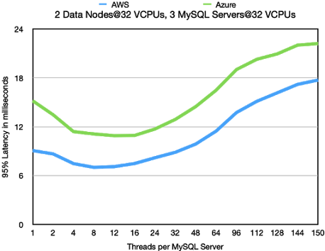
The final setup compares a setup with 32 VCPUs on data nodes and 3 MySQL Servers using 32 VCPUs. This setup mainly focuses on behaviour latency and throughput of MySQL Servers in an environment where the data nodes are not the bottleneck. The test compares AWS with Azure.


We used 3 different benchmarks. Standard Sysbench OLTP RW, this benchmark is both a test of CPU performance as well as networking performance. Next benchmark is the same as OLTP RW using a filter where the scans only return 1 of the 100 scanned rows instead of all of them. This makes the benchmark more CPU focused.


The final benchmark is a key lookup benchmark that only sends SQL queries using IN statements. This means that each SQL query performs 100 key lookups. This benchmark shows the performance of simple key lookups using RonDB through SQL queries.

Conclusions

The results show clearly that AWS has the best latency numbers at low to modest loads. At high loads GCP gives the best results. Azure has similar latency to GCP, but doesn’t provide the same benefits at higher loads. These results are in line with similar benchmark reports comparing AWS, Azure and GCP.


The variations from one benchmark run to another run can be significant when it comes to latency. This is natural since there is a random latency added dependent on how far apart the VMs are within the availability zone. However throughput is usually not affected in the same manner.


In some regions Azure uses several buildings to implement one availability zone, this will affect latency and throughput negatively. In those regions it is important to use Proximity Placement Groups in Azure to ensure that all VMs are located in the same building. The effect of this is seen in the last benchmark results in this report.


The limitations on VM networking are a bit different. This played out as a major factor in the key lookup benchmark where one could see that AWS performance was limited due to network bandwidth limitation. Azure VMs had access to a higher networking bandwidth for similar VM types.


AWS provided the r5n VM types, this provided 4x more networking bandwidth with the same CPU and memory setup. This provided very useful for benchmarking using RonDB data nodes with 32 VCPUs.


Benchmark Results

2 Data Nodes@16 VCPUs, 2 MySQL Server@16 VCPUs

Standard OLTP RW


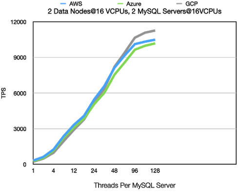
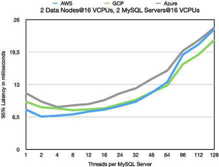
In this benchmark we see clearly the distinguishing features of AWS vs GCP. AWS

has better latency at low load. 6,5 milliseconds compared to 9,66 milliseconds.

However GCP reaches higher performance. At 128 threads it reaches 7% higher

performance at 7% lower latency. So GCP focuses on the performance at high load

whereas AWS focuses more on performance at lower loads. Both approaches have

obvious benefits, which is best is obviously subjective and depends on the application.


This benchmark is mainly testing the throughput of MySQL Servers. The RonDB

data nodes are only loaded to about 60-70% of their potential throughput with

2 MySQL Servers.


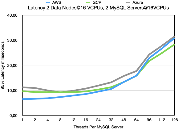
Moving to latency numbers one can see the same story, but even clearer. AWS has

a better latency up to 48 threads where the latency of GCP becomes better. In GCP

we see that the latency at 1 thread is higher than the latency at 12 threads and only

at 24 threads the latency starts to increase beyond the latency at 1 thread. Thus in

GCP the latency is very stable over different loads until the load goes beyond 50%

of the possible throughput. We see the same behaviour on Azure whereas AWS

latency slowly starts to increase at lower thread counts.

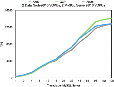
Standard OLTP RW using filter

The OLTP RW using a filter is more focused on CPU performance. The major difference

is seen at higher loads. The latency at low loads is very similar, but at higher loads we

get higher throughput at lower latency. Thus standard OLTP RW has a steeper march

from acceptable latency to high latency. The difference in throughput is very small

between cloud vendors, it is within 10%.


The comparison between AWS and GCP is similar though. The GCP benefit at higher

load is slightly higher and similar to the latency. The AWS advantage at lower loads is

slightly lower. Thus GCP has a slight advantage compared to standard OLTP RW,

but it is a very small difference.

Key Lookups

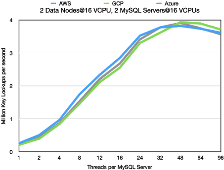
In the graph below we see the number of key lookups that 2 MySQL Servers can drive.

The numbers are very equal for the different cloud vendors. AWS as usual has an

advantage at lower thread counts and GCP gains the higher numbers at higher

thread counts and Azure is usually in the middle.


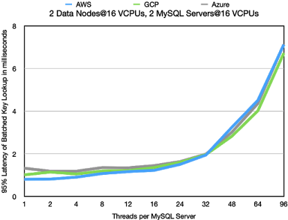
The latency numbers are shown below. These numbers more clearly show the

advantage of AWS at lower thread counts. At higher thread counts the latency

is mostly the same for all cloud vendors. This benchmark is extremely regular

in its use case and thus it is mostly the CPU performance that matters in this

benchmark. Since this is more or the less same on all cloud vendors we see

no major difference.

2 Data Nodes@16 VCPUs, 4 MySQL Server@16 VCPUs

In this benchmark the bottleneck moves to the RonDB data nodes. We now have

sufficient amounts of MySQL Servers to make the RonDB data nodes a bottleneck.

This means a bottleneck that can be both a CPU bottleneck as well as a networking

bottleneck.

Standard OLTP RW
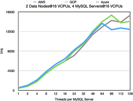

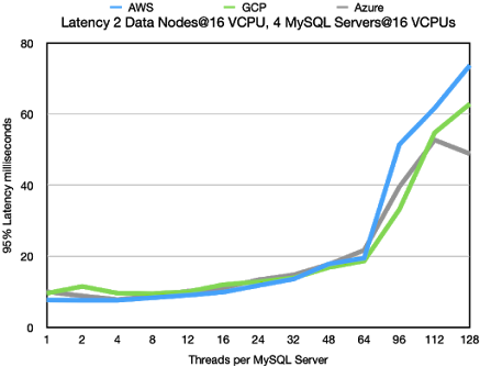
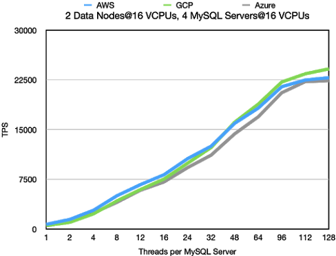
The latency is very stable until we reach 64 threads where we have around 15k TPS at

20 milliseconds latency. At higher thread counts the data nodes becomes the bottleneck

and in this case the latency has a much higher variation. We can even see that latency

at 128 threads in Azure goes down and throughput up. We expect that this is due to

interrupt handling being executed on the same CPUs as database processing happens.

This is something that we will look more into.

OLTP RW using filter

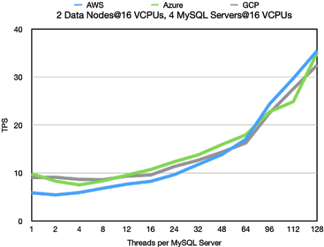
The throughput of OLTP with a filter means that the focus is more on CPU performance.

This makes it clear that the high variation on throughput and latency in standard OLTP RW

comes from handling the gigabytes per second of data to send to the MySQL Servers.

In this benchmark the throughput increases in a stable manner and similarly the latency

goes up in an expected manner.


All cloud vendors are very close to each other except at low thread counts where

AWS have an advantage.

Key Lookups

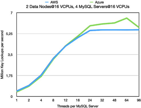
The key lookups with 4 MySQL Server and 2 data nodes and all nodes using

16 VCPUs per node moves the bottleneck to the data node. As usual AWS

wins out on the latency at lower thread counts. But at higher thread counts

AWS hits a firm wall. Most likely it hits a firm bandwidth limitation on the VMs.

This limitation is higher on Azure, thus these VM can go an extra mile and serve

1 million more key lookups per second.

2 Data Nodes@16 VCPUs, 2 MySQL Server@32 VCPUs

This benchmark uses the same amount of CPUs on the MySQL Server side,

but instead of divided on 4 MySQL Servers, it is using 2 MySQL Servers.

We didn’t test GCP in this configuration. We expect no surprises in throughput

and latency if we do.

Standard OLTP RW

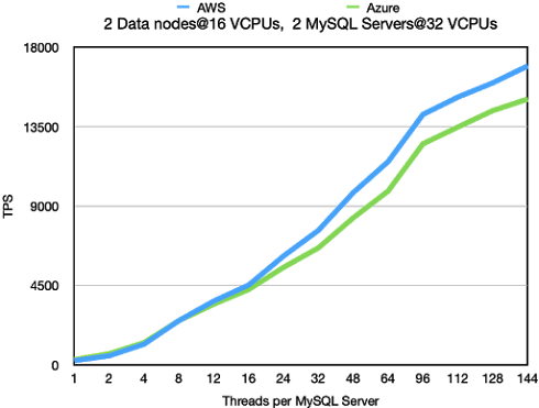
In the Standard OLTP RW we see that the throughput is the same as with

4 MySQL Servers. However the throughput increases in a more regular manner.

What we mainly see is that we can achieve a higher throughput using a smaller

amount of threads in total. This makes the throughput more stable. Thus we

conclude that at least up to 32 VCPUs it pays off to use larger MySQL Servers

if required.


2 Data Nodes@32 VCPUs, 3 MySQL Server@32 VCPUs

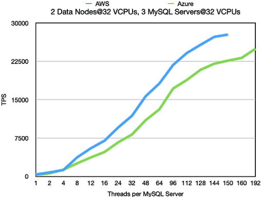
In this benchmark we increased the number of CPUs on the RonDB data

nodes to 32 VCPUs. Most of the testing in this setup has been performed

on AWS. The main reason for including the Azure numbers is because

these numbers show the impact of not using Proximity Placement Groups

in Azure on large regions. We saw clearly in these benchmarks that the

latency in the Azure setup was much higher than in previous benchmarks

that were using a smaller region.


However in the smaller region it was difficult to allocate these larger VMs

in any larger number. We constantly got failures due to lacking resources

to fulfil our requests.

Standard OLTP RW

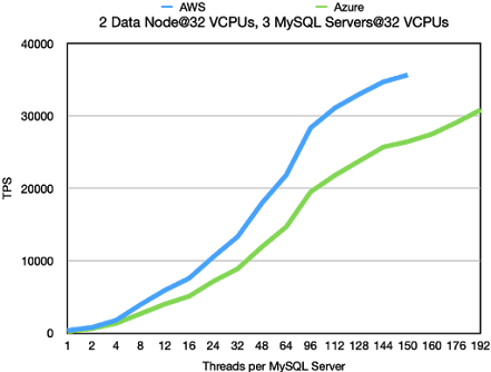
In AWS we discovered that the network was a bottleneck when executing

this benchmark. Thus we used r5n.8xlarge instead of r5.8xlarge VMs in

this benchmark. These VMs reside in machines with 100G Ethernet

connections and each 32 VCPU VM have access to at least 25 Gb/sec

networking. The setup tested here with 3 MySQL Servers doesn’t load the

RonDB data node fully. In other benchmarks we were able to increase

throughput to around 35k TPS. However these benchmarks used a different

setup, so these numbers are not relevant for a comparison. What we see is

that the throughput in this case is roughly twice the throughput when using

16 VCPUs in the data nodes.


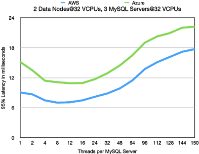
Latency numbers look very good and it is clear that we haven't really

reached the bottleneck really in neither the MySQL Servers nor the

RonDB data nodes.


OLTP RW using filter

Similarly in this experiment we haven’t really reached the bottleneck on neither the

RonDB data nodes nor the MySQL Servers. So no real news from this benchmark.