There are a couple of questions about the blog post on automatic thread configuration in RonDB. Rather than providing an extensive answer in the comment section I thought it was better to answer the questions in a separate blog. In addition I performed a set of microbenchmarks to verify my expectations.
The first question was the following:
ScyllaDB also does something similar with execution stages for better instruction cache. Is this similar to what you're implementing for instruction cache on separating the threads?
The second question is:
I don't really get the functional separation of threads. To execute a query, your data will now go through a pipeline of threads, instead of being executed into one. This means, you need to pass data between 4 threads, until the query is finished. It could be achieved via queueing between threads and wakeups , or maybe spinning to avoid more context switches.
But I do not seem to see what's in that trick. My understanding is that, your query will execute the same number, or more CPU instructions, and since now there is a pipeline of several threads, it will suffer either more spinning, or more cache misses, or more context switches due to this tossing data between threads.
Batch Pipeline vs Thread Pipeline
As an interesting observation there are a lot of similarities to the description here of Software Pipelines with the CPU Pipelines and several CPUs per CPU core.
What I understand from the ScyllaDB description is that it is implemented as an asynchronous engine.
ScyllaDB specifically says that they didn’t want to introduce a Thread Pipeline. Instead they seem to have introduced a Batch Pipeline where they execute one task type at a time. This clearly improves the use of the instruction cache. The Batch Pipeline approach will have best latency when the system is at low load. When the system is at high load the batch size increases and the latency increases. With RonDB and its Thread Pipeline, the latency decreases as the load increases since the likelihood of the thread being awake is higher. Thus RonDB at high load acts as a set of CPUs that interact directly with small messages sent to instruct the receiver of what he is supposed to do. Thus at high load the overhead of switching to a new thread is negligible, there is a small extra cost to handle extra data for the messages, but the messages are small and thus this overhead is small compared to the extra latency introduced by having to wait for another batch to execute before my turn to execute comes.
Actually the Batch Pipeline model resembles the first thread model of NDB Cluster where everything was executed in a single thread. This thread received a batch of messages and executed each of those in FIFO order, the messages sent asynchronous messages to the next part of the code. This actually had exactly the same effect as seen in the Batch Pipeline model since all messages followed the same code path. Thus if 100 messages were received we first executed 100 messages in the transaction block and then 100 messages in the database blocks.
ScyllaDB also handles complex query processing in the same engine. RonDB does all complex query processing in MySQL in a separate program. This enables RonDB to provide a very efficient API in C++, Java and in JavaScript which translates database requests directly into the efficient NDB protocol.
The RonDB model uses a normal FIFO scheduler in each thread and threads only execute a part of the functionality and the database part only executes queries on parts of the database. Thus we achieve both the benefits from the batch processing of similar messages in a pipeline and the division of work into different CPUs.
Microbenchmarking RonDB
RonDB has the ability to execute a benchmark exactly in the fashion as the Batch Pipeline model. This happens when the RonDB data node executes using a single thread. Thus we can use RonDB to analyse how Batch Pipelines compare to Thread Pipelines in a microbenchmark.
In this microbenchmark I run a single RonDB data node without any replication, I run one benchmark program called flexAsynch. This benchmark program sends batches of Inserts, Updates, Reads and Deletes and measures the achieved throughput.
When a read is processed it will be executed in 4 steps, the first step is to receive the network message, the second step handles the transaction processing which ensures that we find the data read and write the correct parts of the data partitions. The third step does the actual read/write of the data, the fourth step sends the data back to the benchmark program.
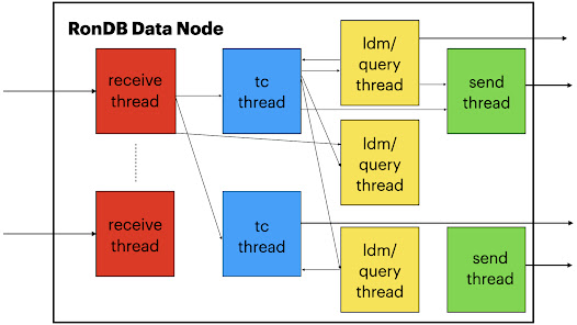
In RonDB using the single-threaded setup the receive part will receive a batch of operations, each of those will be inserted to the job queue in FIFO order.
After executing the receive we will execute those messages that will all execute the transaction part. Each of those transaction part messages will generate a new asynchronous message to be executed by the data owning part. Thus although they are located in the same thread we will still execute all those messages in batches that will all execute the same code and thus achieving the efficiency of the instruction cache in the CPU.
Next all messages will be executed in the data owning part and each of those messages will put something into the send queue which will be the last step executed before we return to the next set of messages in the receive part. Thus in the single threaded configuration of RonDB we get exactly the behaviour of a Batch Pipeline.
The next step is to separate the receive part from the transaction execution part and data owning part. Thus in this case we will have a thread pipeline consisting of two threads.
The third step is to split the thread pipeline into 3 parts. The receive part, the transaction handling part and the data owning part.
The fourth step finally separates the sending part as well into a separate send thread.
All of these steps are easily achieved in RonDB by using a configuration parameter called ThreadConfig.
The expected results here is that the single-threaded variant will get the optimal throughput since it divides the execution based on batches and thus minimizes the instruction cache misses. It is expected that the Thread Pipeline will have the same effect, but spread the work to more than one CPU. In our threaded pipeline we can specify the size of the batches executed before we flush all messages to other threads and before we send them back to the NDB API program.
The results showed that the first step could handle around 750k operations per second. Splitting the receive thread from the other parts improved throughput to around 835k operations per second. The result shows that a fairly small part of the processing happens in the receive stage. The third step to divide the transaction processing step from the data owning part gave a much bigger impact. Here performance increased to 1.5M operations per second.
The fourth step was implemented by specifically disallowing the data owning part and the transaction processing part to not perform any sends. Thus all sending had to happen from a separate fourth thread. This step had very little impact, thus our adaptive send approach where send happens locally if the thread isn’t overloaded and otherwise it is performed by a less loaded thread is a good approach. This means that in RonDB there will be send threads, but for the most part the sending will be done by execution threads that are not so busy. Thus we can use send load to ensure that the CPUs are used in a balanced manner.
What we derive from those numbers is that a Thread Pipeline and a Batch Pipeline has equal efficiency. However the Thread Pipeline provides a lot of benefits. For receive threads it means that the application doesn’t have to find the thread where data resides. This simplifies the NDB API greatly. I have made experiments where the NDB API actually had this possibility and where the transaction processing and data owning part was colocated in the same thread. This had a small improvement of latency at low loads, but at higher loads the thread pipeline was superior in both throughput and latency and thus this idea was discarded.
The Thread Pipeline also improves scalability. As shown here we can have a single thread handling the data owning part and scale this to twice as many operations per second without having to split the data partitions.
I also did an experiment where I used 2 receive threads, 2 transaction processing threads and 2 data owning parts and this scaled nicely to 3M operations per second. What I have noticed is that in larger thread setups it is important that we have sufficient CPU capacity in the receive threads and the transaction processing parts to ensure that the data owning parts execute in an optimal manner. Using 1 receive thread in this setup provides almost the same results, but this architecture gains from having receive threads that can respond quickly such that they can keep the Thread Pipelines busy.
In RonDB there is a configuration parameter called SchedulerResponsiveness. This specifies whether to optimise for latency or for throughput. By increasing the SchedulerResponsiveness we decrease the batch execution sizes before we flush messages to other threads and other nodes.
Thread Pipeline => data partitioning transparent to APIs
From a performance perspective the Thread Pipeline is equally efficient to a Batch Pipeline. However the thread pipeline gives greater flexibility to the architecture. This flexibility is used in RonDB to ensure that many database connections share the same TCP/IP socket. This gives great batching improvements.
Since receive threads execute on behalf of all threads in the data nodes, the API doesn’t have to route the messages to a specific receive thread. Thus normal round robin can be used to spread load if there are several connections from the API to the RonDB data node.
Thread Pipeline decreases the number of data partitions
What we showed here is that the Thread Pipeline enables us to reach the same performance with 2 database threads compared to the 4 that would have been needed if all functionality would be gathered in a single thread. This means that we can handle the same load with half as many data partitions. Decreasing the number of partitions enables us to more efficiently range scans that don’t use the partition key. We also introduced query threads that ensure that one data partition can be read from multiple query threads, thus even more decreasing the need to split data into many partitions. Thus RonDB achieves a nice balance between splitting data partitions for higher write throughput and higher parallelism in range scans with efficiency in performing the range scans.
Thread Pipeline enables Routing of Messages
As mentioned above the Thread Pipeline enables us to route messages from the transaction part to the data owning part. But in RonDB we also have query threads that can read data from several data owning parts. This provides the possibility also for routing based on load in the various threads. Thus thread pipelining not only provides a very efficient approach to executing database requests, it also enables us to build a highly scalable data node that can process many millions of concurrent requests with internal load regulation.
Thread Pipeline versus Batch Pipeline
So based on this analysis we can conclude that the Thread Pipeline and the Batch Pipeline both provide very similar benefits in CPU efficiency. RonDB has seen IPCs of 1.27 in the data owning parts and ScyllaDB reports IPC of 1.31 in their Batch Pipeline.
However the Thread Pipeline at the same time delivers many advantages from a software architecture perspective. It enables transparency of data partitioning, it enables us to decrease the amount of data partitioning required to achieve the performance objectives and it enables us to build very scalable data nodes. RonDB data nodes has shown linear scaling to at least 32 CPUs and it continues to scale to many more CPUs after that and the software is prepared to handle up to 1024 CPUs.
Tossing data between threads
Now to the question about tossing data between threads. The only data transported between threads is the protocol messages. The actual data in the database is handled by the data owning thread. There is one part where the passing of data between threads matters, and this is for sending the message. Sending network messages have a significant overhead in a distributed database and can also cause extra CPU cache misses. RonDB has an additional design requirement that requires collecting messages from several threads to be sent on one socket. Thus sending network messages is a bit special in RonDB. However often we can avoid the extra cost of involving another thread for sending by sending when we have completed a batch of processing.
There is also an adaptive process that moves the CPU processing of sends to the threads with lowest load. Thus in a highly loaded data node we will avoid the sending in overloaded threads to ensure that we can process all the requests coming in.
In addition RonDB uses special handling of large messages, where the large part of the message is transported in a special section. This section is only read by the receiving thread (usually the data owning thread), thus there is no extra cost in passing this part through other threads (usually the transaction processing thread). When received by RonDB from the API this is a simple interpreted program. Messages sent back to the API are sent directly from the data owning part to the API, this message doesn't pass through any Thread Pipeline. Only messages that are part of transaction handling are sent back to the transaction processing part.
Latency in the Thread Pipeline
The next question that one could ask is whether the latency is negatively affected by the thread pipeline. In ScyllaDB they report that the mean execution time for a request is 282 microseconds. This is an eternity when compared to the latency overhead of a thread pipeline. Even if all threads are sleeping when the request arrives, the wakeup latency of a thread is around 5-10 microseconds. So in the absolute worst case there is an added latency of around 15-25 microseconds to execute this thread pipeline.
However in reality the latency at 0% usage is seldom interesting. The latency of interest is the latency that you get when the load starts to reach the highest load. In this case the extra latency that the thread pipeline comes close to zero since most of the threads are awake in this situation.
The total execution time of a key-value lookup in RonDB data nodes is around 2-3 microseconds and writes around 5 microseconds. The thread pipeline means that each thread can execute at maximum speed all the time. An expected latency in a loaded RonDB data node would be on the order of 50 microseconds and thus the overhead of wakeup latencies in this case will be no more than 10% added latency. Compared to the advantages that the Thread Pipeline provides it is a good idea.
Actually this behaviour is of great use in that RonDB becomes more efficient as load increases. Thus if RonDB is overloaded it will become more efficient since the threads will continuously be busy executing the messages and batch effects will increase as the load increases.
Efficiency of the Thread Pipeline
The real performance in a database is not determined by the number of instructions per second. The performance is determined by the number of instructions to execute for an operation divided by the number of instructions executed per cycle. RonDB reaches an IPC of the most critical database code of 1.27. Many other DBMSs have reported numbers in the order of 0.25-0.5. Thus it is clear that the separation of code into a thread pipeline works well.
At the same time we have used many other tricks in RonDB to achieve the desired performance.
One such trick is how we designed our protocols. Most internet protocols are heavy CPU consumers. I had a master thesis student design a generic protocol engine that was intended to be used in NDB. This was probably the most important master thesis project I led. It showed exactly how to NOT do it. When the project was ready and I saw the resulting code, I realised that there is no way to get that code to become efficient. Thus NDB protocols are based on messages where the message data are residing in fixed positions. Thus no protocol processing is required, only copying from the message to data structures used by internal operations.
The code to process those messages can have a lot of instructions, but it is code without any logic, basically just processing fixed data move instructions for the most part. Thus this code is extremely efficient on modern CPUs. In addition the code in RonDB provides hints to the C++ compiler which branches are the normal path through the code. This is important since RonDB is implementing failfast, thus the code is filled with extra assert statements (implemented using a macro called ndbrequire) that will crash the data node immediately if any data is not consistent. All these asserts are also executed in production code to ensure that we don’t continue executing in an incorrect program state. In addition we also constantly generate crash information in the code to be able to understand exactly what happens if there is a failure.
Thus with all the talk about low latency and high throughput, it is important to understand that the highest priority in RonDB is to achieve the highest possible availability.
Instruction Cache
So will our approach decrease the amount of CPU instructions? The answer is no, there will be extra instructions to process the protocol between threads and at times there will be extra CPU instructions to handle context switches. So how can we gain from executing more CPU instructions?
To answer that question I will start by telling a story from my history. I was working in a large company that developed a number of real-time databases in the 1990s. One of those databases was implemented in C++ and aimed at being very efficient. The problem it had was that it used too much generated code and too much code in general. When the code was analysed it was discovered that it spent 5 out of 6 CPU cycles waiting for the instruction cache.
Another story from the 1990s was when I wrote an interpreter for the HW that this company developed. One day I was working on some optimisations, I thought I had done a terrific job, so expected at least 5-10% improvements. I saw 2% decline in performance. After a long day of work I went home very disappointed. Next day I returned and didn’t want to continue working on these things immediately, so I spent some time simply reorganizing the code to get a better flow. Next I ran the tests again not expecting any difference, I was simply verifying that the tests were still working. I saw a 15% improvement. I was very surprised and thought that something must be wrong. However what I found out was that code reordering can have a substantial impact on performance.
This experience I brought with me into the development of NDB and now into RonDB. Thus if you read the code in RonDB you will notice that the code is written such that methods are organised in the flow of execution. Thus using code reordering flags in C++ compilers on the code in RonDB usually leads to worse performance since the code is already organised in an efficient manner.
From the above description I am hoping that the message is conveyed that it is of great importance to avoid executing too much code in a single thread. Decreasing the code size executed in a single thread means that this CPU will be focused on its task.
Thread Pipeline
The thread pipeline always starts with the receive thread. This thread will receive the request from the network. By providing this as a separate thread we provide the ability to colocate the operating system network processing with the processing by the receive thread itself. I covered this in a blog in 2016. Linux provides the ability to handle the network processing in the same CPU as the recv call is made in. This enables very efficient handling of the receive part of the network processing.
There is another reason why the receive part is required to be a separate thread in RonDB. This is because one socket can be used to carry thousands of simultaneous connections to the data node. Thus the receive part will break the received messages into the smaller messages and these smaller messages will be transported on memory channels to the appropriate thread. Thus one TCP/IP receive that receives say 32 kByte of data can easily be broken into 300 separate messages to be executed by different threads.
You can think about this thread pipeline as an example of a programmer using an assembly line. By dividing the tasks into smaller tasks we decrease the size of the program each task will have to execute. The total program grows a little bit, but since each thread will only see the part it is responsible for it will have very good code locality.
If you think of CPUs as workers in the assembly line, it is also important to not switch workers. To avoid that RonDB uses CPU locking to avoid that the OS all of a sudden decides to move the execution to another CPU. The cost of rebuilding the CPU caches in a new CPU can take quite a few microseconds. In our case even most context switches avoid this cost since most of the time there are no other tasks waiting to be executed on this CPU since we have separated the heavy CPU consumers into different CPUs. Thus even after returning from a context switch we will have fairly hot CPU caches.
The thread pipeline also splits the data cache usage. The LDM threads that handle database operations have no data stored on global transaction state and have no knowledge about the global transaction state.
Thus the thread pipeline provides both an improved use of the instruction CPU cache as well as the CPU data caches.

